A Running the Code

A.1 Interactive Execution

Our recommended IDEs follow those stated in the Preface: Positron, which handles both R and Python; RStudio, which remains a solid choice for R alone; and IDLE, the bare bones Python option. There are certainly fancier development environments. But, these are relatively simple and do the job. Code can be loaded and run interactively from the console command line. This is a plus because interactive execution encourages experimentation. Simulation studies are rarely run once. Parameters change, bugs are corrected, and new questions emerge during the analysis. Working directly from the console provides a workflow that supports this exploratory process.

To work interactively one loads the function of interest into the console with source in R and import in Python and then runs the program by entering the function’s name with its associated arguments. For example, in R

source("sim_template.R")
out <- sim_template(1234, 100, 20, 4, 5)
lapply(out, round, 3)

## [[1]]
## [1] 5.930 4.992 4.470 4.336 4.306
##
## [[2]]
## [1] 4.627 6.108 4.543 4.708 4.395
##
## [[3]]
## [1] 5.243 5.121 4.692 4.362 3.357
##
## [[4]]
## [1] 4.281 7.403 5.368 5.100 5.264

repeats, with rounded output, our Cauchy example of Section 3.3. Similarly in Python

import numpy as np
from sim_template import sim_template
out = sim_template(1234, 100, 20, 4, 5)
np.round(out, 3)

## array([[5.621, 5.955, 5.26 , 4.612, 5.325],
##        [4.698, 5.995, 6.151, 5.02 , 5.016],
##        [5.352, 6.227, 4.562, 5.257, 5.833],
##        [4.806, 5.437, 4.913, 5.42 , 5.474]])

recreates (with rounding) the Cauchy example from Section 4.3.

A caveat here is that you must be in the directory that contains the file you source or import. In R you use getwd and setwd to find and set the current working directory. For Python you must first import the os module and then the parallels of the R commands are os.getcwd and os.chdir.

In the book’s code repository the R and Python scripts live in R/ and python/ subdirectories, so “the directory that contains the file” means one of those two after cloning. Each of these directories contains a copy of sim_worker — holding the \(\pi\) worker, our first running example — alongside the named workers for the other examples (IQR_worker.R, regression_worker.R, cauchy_worker.py, epidemic_worker.py, and so on). To reproduce a particular example, copy the corresponding named worker over sim_worker.R or sim_worker.py and run sim_template as shown above; the Cauchy transcripts in this appendix were produced exactly that way, with the contents of IQR_worker.R standing in as sim_worker.R.

For the purist we should observe that there is one “IDE” that everyone likely has where both R and Python code can be executed: namely, the terminal (MacOS and Linux) or Windows terminal (Windows). Set the shell directory to the place where your code resides. Then, enter R or python3 on the command line to start an R or Python session. After that the source/import commands will load your code and you can run it directly.

A.2 Plotting Epidemic Trajectories

It’s hard to appreciate the material in Chapter 6 without pictures. The numbers in the output from epidemic_driver are overwhelming unless they are summarized in some way and it’s hard to beat a picture when it comes to that. The code below will take the output from epidemic_driver, the number of the processes/towns and an optional file name as input and create a plot of the data with a specified name (i.e., f_name).

from epidemic_driver import epidemic_driver
import numpy as np
import matplotlib.pyplot as plt

def plot_epidemic(history, f_name = None):
    # convert list to array
    history = np.array(history)
    if history.ndim == 3:
        history = np.vstack(history)
    days = np.arange(history.shape[1])
    for i in range(history.shape[0]):
        plt.plot(days, history[i, :], alpha=0.2)

    plt.xlabel("Day")
    plt.ylabel("Infected")
    plt.title("Epidemic trajectories")
    plt.savefig(f_name, dpi=300)
    plt.show()

if __name__ == "__main__":

    town = 3  # process to plot
    out = epidemic_driver(
        1234, # seed
        30,   # days
        30,   # n_reps
        4,    # n_cores
        1000, # pop_size
        20,   # initial_infected
        0.05, # death_prob
        5,    # contacts_per_day
        3,    # recovery_days
        10,   # n_migrants
        0.05, 0.15, 0.25, 0.30 # infection_prob
    )

    plot_epidemic(out[town], "epidemic_plot.png")

By modifying the epidemic parameters you can see how they affect trajectories. The program is currently set to show the trajectories for process 3.

Running the code from the terminal goes something like this. First, enter this on the command line:

% python3 plot_epidemic.py

Wait a few seconds and your plot will appear. If you have furnished a file name to plot_epidemic a hard copy of the figure will appear in the shell’s working directory. In this case it is a file named epidemic_plot.png. That is what is shown in Figure A.1.

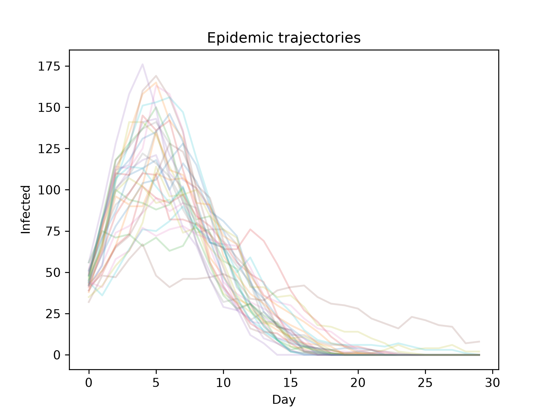
Figure A.1: Epidemic trajectories

As noted in Chapter 4 any Python script that creates a Pool, Manager, or other multiprocessing object should protect executable code with an if name == “main”: block. This is particularly important on macOS and Windows, where child processes are started using the spawn method. Running this code directly from the terminal without the guard will create a chain of spawned processes, hang up and never finish.