3 Parallel Simulation in R

A basic premise of this book is that for some purposes you want a plug-in-and-go “formula” you can fit into your workflow without getting bogged down in extraneous details. Running simulation experiments usually falls into that category and to run them expeditiously on your personal machine will almost surely require exploiting its multiple cores effectively. With that in mind we now present a flexible scheme for doing parallel simulation experiments in R. You’ll meet our first incarnation of sim_template, a concise extensible R function that creates a local cluster of processes on your computer and sends out simulations to be done across multiple worker processes. In Section 3.1, we give a listing of sim_template and briefly discuss its use, so you can quickly get code up and running. We follow this with two small examples in Sections 3.2 and 3.3 that illustrate using the code. Timing experiments are also carried out to see the speed-up provided by a parallel treatment. We conclude with a read-optional section about how sim_template works and the specific choices that were made in its construction.

3.1 sim_template.R

The setting is that of Chapter 2. We have an estimator \(\hat\theta\) of a parameter \(\theta\) and want to conduct a simulation study to learn how it can be expected to perform in practice. The estimator will be computed on each of n_reps simulated samples of size n. Usually n_reps is large, so we get a clear picture of how the estimator behaves, and n is modest, set by what a real study would collect. The listing that follows parallelizes that n_reps-fold simulation computation across the processors of a personal machine.

Listing 3.1. R simulation template.

sim_template <- function(seed, n, n_reps, n_cores, ...){

  # load libraries
  library(parallel)
  library(dqrng)

  # import the worker program
  source("sim_worker.R")
  
  # set the seed for use with R's random number generator  
  set.seed(seed)
  
  # replications to be distributed 
  base_reps <- n_reps %/% n_cores
  remainder <- n_reps %% n_cores
  reps <- rep(base_reps, n_cores)
  
  # load balance
  for(i in seq_len(remainder)) reps[i] <- reps[i] + 1
    
  # integer seeds and increments for each process
  sv_list <- generateSeedVectors(n_cores)
  stream_list <- generateSeedVectors(n_cores)

  # parameters lists for the simulation experiment
  set_up <- vector("list", n_cores)
  for(i in 1:n_cores){
      set_up[[i]] <- list(
      n_reps = reps[i],
      stream = stream_list[[i]],
      seed   = sv_list[[i]])
      }
  
  # create the cluster
  cl <- makeCluster(n_cores)
  on.exit(stopCluster(cl), add = TRUE)
  
  # send information to the worker processes
  clusterExport(cl, c("worker", "n"), envir = environment())
  clusterEvalQ(cl, library(dqrng))
  clusterEvalQ(cl, dqRNGkind("pcg64"))
  
  # apply worker to the set_up list elements
  result <- parLapply(cl, set_up, function(worker_setup) {
    worker(n, worker_setup, ...)
     }
  )
  
  # return output
  result
}

To use sim_template it suffices to merely understand its function signature:

sim_template(seed, n, n_reps, n_cores, ...)

The arguments are

• seed: your personal choice for the seed to initialize the simulation,

• n: the sample size,

• n_reps: the desired number of replicate samples of size n,

• n_cores: the number of worker processes to be used in the simulation,

• the optional ... argument that provides the highway for passing information about model parameters to the worker functions.

The remaining piece of the puzzle is a worker function that is assumed to be in an R script sim_worker.R that will be imported by sim_template. This function constructs data from a parametric model involving \(\theta\) and computes an estimator of \(\theta\) for a collection of samples from the model. This is where your input comes in. The next listing gives a generic sketch of how sim_worker.R might appear where “YOUR CODE GOES HERE” corresponds to the code you must write that computes the estimator of \(\theta\) for a sample of size n from the model of interest.

worker <- function(n, set_up, ...){
  # unbundle the simulation parameters
  n_reps <- set_up$n_reps
  stream_1 <- set_up$stream[1]
  stream_2 <- set_up$stream[2]
  seed_1 <- set_up$seed[1]
  seed_2 <- set_up$seed[2]
  
  # set the seed and increment of the generator
  dqset.seed(c(seed_1, seed_2), c(stream_1, stream_2)) 
  
  # unpack the model parameters 
  param_list <- list(...)
  
  # array of uniforms
  U <- matrix(dqrunif(n * n_reps), nrow = n, ncol = n_reps)
  
  result <- apply(U, MARGIN = 2, FUN = function(u) {
      YOUR CODE GOES HERE
    })
  result
}

This code uses information in the list set_up passed in from the calling program (i.e., sim_template) to seed a random number generator from the dqrng package that is discussed in Appendix C. Then, it creates a matrix of uniform random deviates via dqrunif: the dqrng package’s random uniform generator.

The columns of the matrix U represent samples of size n from the uniform distribution. R’s apply function is used to transform these uniforms to samples from the focal parametric model and then compute a corresponding parameter estimator.

To be specific, in place of the “YOUR CODE GOES HERE” part of worker you’ll need to enter R code that

• creates data from your target parametric model using parameter values passed in to sim_template in the ... argument and

• computes the parameter estimator for each data set simulated from your model.

The sim_worker.R script is assumed to reside in the same directory as sim_template. If that is not the case, then the source("sim_worker.R") line of sim_template needs to be altered to

source("/path_to_sim_worker/sim_worker.R")

with /path_to_sim_worker the directory path to the sim_worker.R script. Also, it is assumed that the dqrng random number generator has been installed. If not enter install.packages("dqrng") on the R console command line.

3.2 Estimating \(\pi\)

Most people know that \(\pi\) is about 3.14, and R will print a few more digits if you ask for pi. But \(\pi\) is irrational: its decimal expansion never ends and never repeats. So, we can only ever estimate it.

In Chapter 2 we considered estimating \(\pi\) by throwing darts at a square with a circle drawn inside. The resulting estimator was four times the fraction of darts that landed in the circle.

We now wish to carry out a computer simulation of the dart throwing experiment. To do that one generates random dart coordinates as pairs of numbers in the interval \([-1, 1]\) and keeps track of the pairs that fall inside the unit circle. Following the recipe from Chapter 2, each simulated replication corresponds to n dartboard throws and the estimate of \(\pi\) for that replication is the observed in-circle fraction of hits times four.

An R script that performs the estimation operation is given below.

worker <- function(n, set_up) {
  
  # unpack the parameters
  n_reps   <- set_up$n_reps
  stream_1 <- set_up$stream[[1]]
  stream_2 <- set_up$stream[[2]]
  seed_1   <- set_up$seed[[1]]
  seed_2   <- set_up$seed[[2]]
  
  # set the seed and stream
  dqset.seed(c(seed_1, seed_2), c(stream_1, stream_2))
  
  # generate matrices of uniforms on [-1, 1] 
  x <- matrix(dqrunif(n * n_reps, min = -1, max = 1), nrow = n, 
              ncol = n_reps)
  
  y <- matrix(dqrunif(n * n_reps, min = -1, max = 1), nrow = n,
              ncol = n_reps)
  
  # estimate pi for each replication
  pi_hat <- 4 * colMeans(x^2 + y^2 <= 1)
  
  pi_hat
  }

Reading the worker listing one line at a time, we see this is just the Chapter 2 algorithm spelled out in R code. First we use set_up to obtain the value of n_reps as well as the seeds and increments for the PCG64 generator that make its particular stream distinct from those for other worker processes. Then,

dqset.seed(c(seed_1, seed_2), c(stream_1, stream_2))

instantiates the worker’s random number stream. This adheres to the advice of Chapter 2 and carefully selects each stream’s parameters.

Next

  x <- matrix(
    dqrunif(n * n_reps, min = -1, max = 1),
    nrow = n,
    ncol = n_reps
  )
  
  y <- matrix(
    dqrunif(n * n_reps, min = -1, max = 1),
    nrow = n,
    ncol = n_reps
  )

draws all the random numbers the worker needs to do its computations. The x and y array entries represent the pair of dart coordinates in the interval \([-1, 1]\) for each replication. Then, the snippet

pi_hat <- 4 * colMeans(x^2 + y^2 <= 1)

puts everything together. It computes a logical array with TRUE for points that fall in the circle and FALSE otherwise. The logicals evaluate numerically as 1 and 0 respectively so that colMeans returns the proportion of hits in the circle for that particular replication or column. Finally pi_hat is returned as an n_reps long vector, with one estimate per replication.

An alternative way to compute the \(\pi\) estimators here is

# Identify points inside the unit circle
inside <- x^2 + y^2 <= 1

# Estimate pi by applying the mean function to each column
pi_hat <- 4 * apply(inside, MARGIN = 2, FUN = mean)
  

This is quite acceptable; but, it is slow relative to the colMeans approach.

The apply function is syntactically convenient. Still, it is no better than writing explicit loops from a performance perspective. It extracts each column of the target array and calls the R mean function separately. When the matrix contains many columns, the repeated R-level function calls and creation of temporary objects imposes substantial overhead.

In contrast, colMeans takes the entire logical array as an argument and evaluates it using underlying compiled code. This is called vectorization and is very fast. To be clear, the looping must take place somewhere. But, colMeans moves it from the R interpreter to underlying compiled code.

Many functions in R have been vectorized. These include math transformations, logical comparisons, and arithmetic. So, an expression like inside <- x^2 + y^2 <= 1 is vectorized and is array aware in that it maintains the matrix dimensions. While the function mean will take arrays as arguments it returns but a single number and must be explicitly applied column-wise for this problem.

There is a useful lesson here that will appear again in Chapter 8. Parallelization is not the first or only source of speed. Efficient serial work inside each process still matters. Adding cores to a computation that makes hundreds of thousands of interpreted function calls merely distributes inefficient work.

Running the code produces results like

mean(unlist(sim_template(1234, 100, 1000000, 4)))

## [1] 3.141554

This averages one million replications, each a collection of 100 virtual dartboard experiments, run across four cores. The square-root law from Chapter 2 is at work here in that a hundred million dart throws bought us only about four decimals of accuracy.

Some timing experiments (using R’s bench library) produced results like those in Table 3.1. What is being shown there is the median execution time, across ten consecutive runs, for sim_template with the \(\pi\) estimation worker when the sample size is 100, the number of replications is 1,000,000 and anywhere from 1 to 8 processes are employed for the computation. Two machines were used for comparison: an 8 core iMac and a 20 core ASUS laptop. The iMac has 4 performance and 4 efficiency cores while the ASUS has 8 performance and 12 efficiency cores.

We obtain a modest increase in speed by going from serial to parallel with up to 4 processes. Going beyond 4 actually results in slower execution.

Table 3.1: Table 3.2: Median elapsed execution times (seconds) for the parallel \(\pi\) simulation. Interquartile ranges are shown in parentheses. Speedup is computed relative to the one-core execution on the same machine.

Cores	iMac M4 Median (IQR)	Speedup	ASUS i7 Median (IQR)	Speedup
1	1.696 (0.036)	1.000	1.750 (0.105)	1.000
2	1.231 (0.132)	1.378	1.030 (0.040)	1.699
3	1.113 (0.054)	1.524	0.880 (0.258)	1.989
4	0.990 (0.021)	1.714	0.790 (0.217)	2.215
5	0.992 (0.279)	1.711	0.965 (0.433)	1.813
6	1.022 (0.074)	1.659	0.800 (0.265)	2.188
7	1.001 (0.020)	1.694	0.930 (0.130)	1.882
8	1.093 (0.108)	1.551	0.820 (0.157)	2.134

One measure of performance in parallel computing is speed-up. This is the ratio of the serial time to run a program to the time it takes to run it with n_cores processes. The ideal case is linear speed-up which evaluates as just the number of workers. So, for example, with 4 worker processes the best possible speed-up is 4: the code runs 4 times faster. In practice linear speed-up is seldom attainable.

The best speedup for the iMac was 1.714 using four processes, while the best speedup for the ASUS was 2.215, also using four processes. Thus, parallelization made the computation about 1.7 times faster on the iMac and 2.2 times faster on the ASUS.

These timing results are a bit disappointing but not unexpected. The problem is too small for a parallel treatment. For parallelization to produce substantive results the worker function must do something that takes time. Here it’s doing only a simple numerical calculation. However, to get to that point the cluster must be started which entails starting separate R sessions for each of the worker processes followed by loading and exporting objects/functions to the workers. Then, the data must be sent to each worker and, once the workers have finished their appointed tasks, the results must be collected and the cluster must be shut down. In brief, there is a lot of time consuming overhead involved that has nothing to do with the problem at hand. The next example gives an instance where going parallel pays a somewhat higher dividend.

3.3 Cauchy Data

In underwater acoustics random “pops” or noise bursts from sources such as marine life, equipment, or geological activity produce occasional spikes in the received signal strength. We can model these amplitude outliers with a Cauchy distribution. Then, simulation experiments allow us to explore such things as detector thresholds and false-alarm rates in sonar arrays.

To use sim_template in this setting we must generate data by sampling from a Cauchy distribution with \(\theta\) a scale parameter that must be estimated. An estimator one might consider in this setting is half of the sample interquartile range (IQR).

Why the IQR instead of something more familiar? The mean and standard deviation for the Cauchy distribution do not exist and their sample parallels are unstable statistics. In contrast the sample IQR remains an interpretable, well-behaved summary measure.

An appropriate sim_worker function for the Cauchy case might now take the form

worker <- function(n, set_up, ...){
  # load the library
  library(matrixStats)
  
  # unbundle the simulation parameters
  n_reps   <- set_up$n_reps
  stream_1 <- set_up$stream[1]
  stream_2 <- set_up$stream[2]
  seed_1   <- set_up$seed[1]
  seed_2   <- set_up$seed[2]
  
  # unpack the value of the scale parameter
  param_list <- list(...)
  theta <- param_list[[1]]
  
  # set the generator seed and increment
  dqset.seed(c(seed_1, seed_2), c(stream_1, stream_2)) 
  
  # array of random uniforms
  U <- matrix(dqrunif(n * n_reps), nrow = n, ncol = n_reps)
  # quantile transformation
  X <- theta * tan(pi*(U - .5))

  # columnwise quartiles
  Q <- matrixStats::colQuantiles(X, probs = c(0.25, 0.75), type = 7)

  # scale estimates
  theta_hat <- 0.5 * (Q[, 2] - Q[, 1])

  theta_hat
}

The first step in this listing coincides with our sim_worker sketch and the \(\pi\) worker development in particular where we use the information in set_up to set the seed and increment of the generator.

Following along with the generic simulation worker outline the next steps are to extract the model parameter (in this case the specified value of theta) from the ... argument and create an array U containing all the uniform random numbers that will be used in the simulation. This array is then transformed to Cauchy values using the explicit form for the Cauchy quantile function \(Q(u) = \tan(\pi (u - .5))\) and the input value for theta.

You might think of theta as a trial scale parameter value. Then, the quantile transformation produces data from a postulated Cauchy scale parameter model and we can use sim_template to assess the performance of the interquartile range based estimator for that particular parameter choice.

Now there are several options and, if we follow the sim_worker formula, we would proceed to

Q <- apply(X, MARGIN = 2, FUN = quantile, prob = c(.75, .25))
theta_hat <- .5*(Q[1,] - Q[2,])

which computes the first and third sample quartiles of the columns of the X array and then takes their difference to get the column-wise interquartile ranges. This is perfectly satisfactory and a solution using apply that works quite generally. But, it is slow relative to another option that exists in this case.

The colQuantiles function from the matrixStats package

install.packages("matrixStats")

is designed specifically for column-wise matrix calculations. It accepts the entire matrix in one call and performs the column iteration in optimized compiled code. Both expressions compute the same quartiles; but colQuantiles does so much more efficiently.

To run sim_template in this setting one might enter, e.g.,

sim_template(1234, 100, 20, 4, 5)

## [[1]]
## [1] 5.929604 4.991993 4.470474 4.336315 4.306422
##
## [[2]]
## [1] 4.626911 6.108323 4.542509 4.707605 4.394840
##
## [[3]]
## [1] 5.243493 5.121492 4.692002 4.361764 3.357274
##
## [[4]]
## [1] 4.280723 7.402930 5.367711 5.099618 5.264122

This produces 20 estimators (5 per process) of \(\theta\) from samples of 100 Cauchy random variates.

Observe that the ... argument of sim_template has now been replaced by 5. This is passed on to become the value of the corresponding argument for worker. So, 5 is the value and sole component of the param_list variable in sim_worker and we are assessing how well our scale parameter estimator performs when the true scale parameter is 5.

Some timing experiments produced results like those given in Table 3.3. Realistically, this problem is too small to merit a parallel treatment and one has to boost the number of samples fairly high to get any benefit out of using more than one worker process. Still, when the number of samples is large enough there is a substantial time improvement and even the efficiency cores appear to contribute at a somewhat reduced rate. The maximum speedup is about 3.2 on the iMac using six processes and 4.7 on the ASUS using eight processes.

Table 3.3: Table 3.4: Median elapsed execution times (seconds) for the parallel Cauchy simulation. Interquartile ranges are shown in parentheses. Speedup is computed relative to the one-core execution on the same machine.

Cores	iMac M4 Median (IQR)	Speedup	ASUS i7 Median (IQR)	Speedup
1	11.73 (0.14)	1.00	10.82 (0.08)	1.00
2	7.76 (0.08)	1.51	5.59 (0.05)	1.94
3	5.87 (0.11)	2.00	4.03 (0.77)	2.68
4	4.48 (0.14)	2.62	3.24 (0.27)	3.33
5	4.21 (0.10)	2.79	2.84 (0.22)	3.81
6	3.68 (0.08)	3.18	2.54 (0.30)	4.26
7	3.72 (0.03)	3.15	2.33 (0.17)	4.65
8	3.85 (0.05)	3.05	2.31 (0.16)	4.68

Figure 3.1 shows a histogram created using a million sample IQRs from samples of size 100 obtained using sim_template with the Cauchy version of sim_worker and \(\theta = 5\). Theory predicts our cloud of IQR values should look like a normal cloud centered at 5 with variance 0.6 for large values of n. An overlay of this particular normal density is shown with the histogram from which one might conclude that samples of size 100 are not large enough for the normal approximation to be very precise in the upper or lower tails of the IQR sampling distribution.

Looking back it is worthwhile to contrast the objectives of our two examples. The estimation of \(\pi\) was primarily a vehicle for introducing parallel simulation and independent random-number streams. The underlying Binomial model there is well understood and exploring the sampling distribution would provide little new information. This is why we gave it rather limited attention. In contrast, the Cauchy example illustrates one of the principal uses of simulation: investigating the finite-sample behavior of estimator sampling distributions when asymptotic theory may be suspect or unreliable.

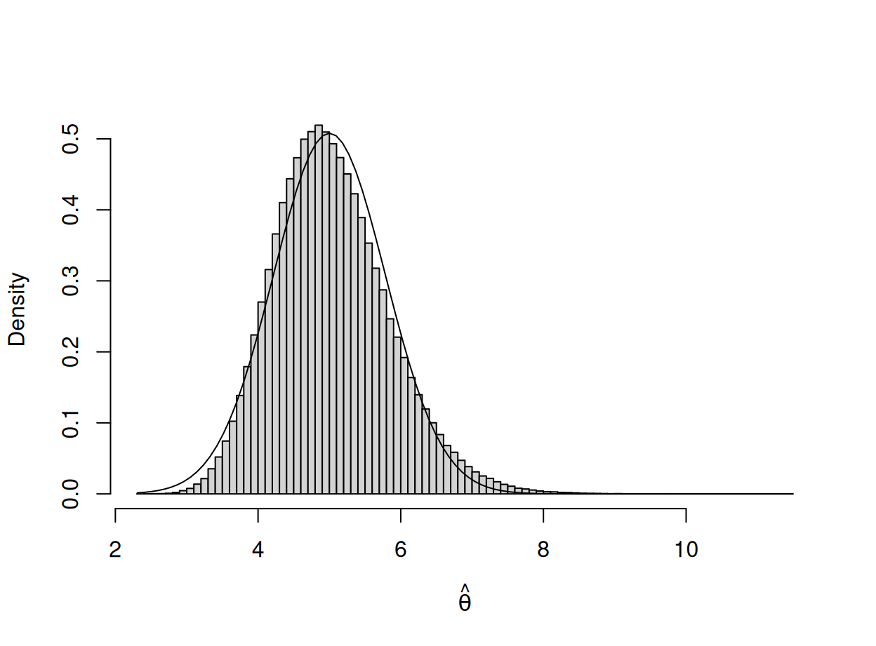
Figure 3.1: Histogram of 1,000,000 Cauchy Scale Estimators

Well, that’s all there is to it. Now you can create your own sim_worker.R script and simulate away.

In the next section we discuss sim_template in detail. But, if that isn’t of interest to you, skip ahead to Chapter 5 where the use of sim_template is more thoroughly illustrated.

3.4 Program Details

We now explain the workings of sim_template. To accomplish this it will be helpful to start with a serial version of the program: namely,

sim_template_serial <- function(seed, n, n_reps, ...){
  # import the worker function
  source("sim_worker.R")
  
  # set the seed for R's random number generator
  set.seed(seed)
  
  # set up the rng
  library(dqrng)
  dqRNGkind("pcg64")
  
  # lists holding the integer seed and increment
  sv_list <- generateSeedVectors(1)
  stream_list <- generateSeedVectors(1)

  # information for the worker
  set_up <- vector("list")
  set_up <- list(
    n_reps = n_reps,
    stream = stream_list[[1]],
    seed = sv_list[[1]]
  )

  worker(n, set_up, ...)
}

So, let us initially dissect this listing.

The program sim_template_serial begins by importing the R script, sim_worker.R that creates the data and computes the estimators. The next step is to set the seed for the R random number generator. This is accomplished with set.seed(seed) that also serves to set the initial seed for the dqrng library that we subsequently load. This library contains our preferred PCG64 random number generator. Then,

  sv_list <- generateSeedVectors(1)
  stream_list <- generateSeedVectors(1)

  set_up <- vector("list")
  
  set_up <- list(
    n_reps = n_reps,
    stream = stream_list[[1]],
    seed = sv_list[[1]]
  )

creates a list, set_up, that holds the number of samples to be generated and the values that are needed to set the seed and the increment for the PCG64 generator. This information is passed on to the worker function in the statement

  worker(n, set_up, ...)

Note that the ... argument to sim_template_serial is also sent on to worker. Recall we used this to set the value of the scale parameter in the Cauchy example of the previous section and this is its purpose more generally: namely, to specify the values of the model parameters that will be used in the simulation experiment.

Once worker receives the information in set_up it uses those details to set the seed and increment of the PCG64 generator via the dqset.seed function from the dqrng package. The ... argument is turned into a list of model parameters and the n by n_reps array of uniform random samples is created. The body of the worker function would therefore contain code of the form

  # unbundle the simulation parameters
  n_reps <- set_up$n_reps
  seed   <- set_up$seed
  stream <- set_up$stream
  
  # unpack the model parameters
  param_list <- list(...)

  # set the seed and increment
  dqset.seed(c(seed[1], seed[2]), c(stream[1], stream[2]))
  
  # array of random uniforms 
  U <- matrix(dqrunif(n*n_reps), n, n_reps)

Now let us deal with sim_template: the parallel version of sim_template_serial. The basic task has not changed. We want to obtain n_reps estimator values computed from samples of size n. But, the work will now be broken into chunks that will be handled by the individual worker processes.

The start of sim_template is much the same as for sim_template_serial except that we load the parallel package to allow us to do parallel computations. These library calls sit inside the function deliberately: they keep sim_template self-contained, and the same convention lets each worker function carry its own package dependencies to the worker processes. Things change when we get ready to allocate tasks to the workers. If n_reps is a multiple of n_cores, then each process will compute the estimator for n_reps/n_cores samples. But, that will not always be the case and there may be some left-over samples to be treated. Specifically, there may be a non-zero value for

remainder <- n_reps %% n_cores

If this is not zero, it needs to be allocated across the workers in a way that balances the workload. The next bit of code carries out that operation:

  base_reps <- n_reps %/% n_cores
  remainder <- n_reps %% n_cores
  reps <- rep(base_reps, n_cores)
  
  # load balance
  for(i in seq_len(remainder)) reps[i] <- reps[i] + 1

This code block begins by creating an array composed of the base value returned after integer division of n_reps by n_cores. If there is no remainder in this division we are done and each worker treats base_reps replications. On the other hand, a nonzero remainder causes the number of replications for the first remainder processes to be augmented by one.

The next step is to find seeds and increments for each worker process that produce distinct streams. If there are n_cores processes to do the work we will need a separate seed and increment for each one’s random number generator. The code

  sv_list <- generateSeedVectors(n_cores)
  stream_list <- generateSeedVectors(n_cores)

produces what we require for that purpose. We bundle this information together in what is now a list of lists:

  # list to hold the simulation parameters 
  set_up <- vector("list", n_cores)
  for(i in 1:n_cores){
    set_up[[i]] <- list(
      n_reps = reps[i],
      stream = stream_list[[i]],
      seed   = sv_list[[i]]
    )

The second and third elements of set_up contain what will be used for the generator’s seed and increments.

We are now ready to start (and stop) the cluster via

  cl <- makeCluster(n_cores)
  on.exit(stopCluster(cl), add = TRUE) 

which first creates a cluster of n_cores workers. Whenever sim_template ends (either by plan or through an error) the on.exit function will be triggered and the cluster will be shut down. This ensures that there are no orphaned processes left running.

To provide each process with the information it needs to do its work, we use

  clusterExport(cl, c("worker", "n"), envir = environment())
  clusterEvalQ(cl, library(dqrng))
  clusterEvalQ(cl, dqRNGkind("pcg64"))

This sends the sample size and worker function to all the worker processes, calls the dqrng package and sets the random number generator as PCG64 on all the nodes.

The work is now distributed across the cluster using a parallel version of R’s lapply function:

  result <- parLapply(cl, set_up, FUN = function(set_up_list) {
    worker(n, set_up_list, ...) } )

This transmits the appropriate sub-lists from set_up to the individual processes and applies the worker function to each of them. Just as with sim_template_serial this information is used to set the seed and the increment of that process’s particular version of PCG64 in sim_worker and produces an array of uniform random numbers determined by n and the number of replicate samples.

The worker program performs its task and reports the outcome back to the main program when it is finished. This information is collected up and returned in result, which contains n_cores vectors of values for the estimators. At that point sim_template has concluded its work.

3.5 A Note on Apply vs. Tidyverse

If most of your R has been written with the tidyverse, the apply family used here may look old-fashioned. It is worth explaining why we chose it rather than one of the newer alternatives.

What lapply does is simple: it takes a list and calls a function on each of its components. parLapply follows the same pattern but distributes the list elements among a cluster of worker processes. Because the replications in a simulation are independent, “run this function on each chunk” is exactly the operation we need. The parLapply call also maps directly onto the parallel recipe from Chapter 2.

The apply family can serve two different purposes in our simulation code. Inside sim_template, parLapply is the parallel engine: it takes the list of per-process setups and runs the worker on each one in a separate process. Within a worker, a calculation may also need to be performed separately on every column of a matrix, with each column representing one simulated sample. The general-purpose expression apply(X, MARGIN = 2, FUN = f) provides a concise way to do this. Convenience does not necessarily imply maximum efficiency, however. apply extracts the columns of its array argument and calls f repeatedly. When an appropriate specialized vectorized function exists, it is generally preferable. For example, the \(\pi\) worker uses colMeans rather than apply(X, 2, mean) and the Cauchy worker uses matrixStats::colQuantiles rather than apply(X, 2, quantile). The specialized functions perform more of the columnwise work in optimized compiled code.

The tidyverse also provides tools for iteration, notably purrr::map() and related functions. The furrr package can run this style of code in parallel using the future framework. We do not use those tools here for two reasons. First, apply is part of base R, and the parallel package containing parLapply is included with R. Although our simulations require packages such as dqrng and matrixStats, no additional iteration or parallel-processing framework is needed. Second, an explicit cluster keeps the workers, chunks, and transfer of information visible which is our preference.

None of this is a verdict against the tidyverse, which provides excellent tools for data manipulation and functional programming. Readers who want to learn it properly will find a friendly, example-driven treatment in Ismay et al. (2025).

The strongest reason for our approach is that the relevant correctness issues remain out in the open. When work is split among processes, the subtle part is not the splitting but giving each process an independent random-number stream—the exact pitfall discussed in Chapter 2. Building the cluster explicitly keeps the seeding operation next to the code that uses it.

The future ecosystem also supports statistically sound parallel random-number generation, while doRNG provides reproducible random-number generation for foreach computations. These frameworks handle the machinery at a higher level of abstraction. For a book that aims to show the moving parts, we choose to keep that machinery on the page. In production code built on a familiar framework, the opposite tradeoff may be more appealing.

When should you reach for the other tools? One important case is when you want the same code to run sequentially, across the cores of a laptop, or on a computing cluster by changing only the backend. That portability is one of the purposes of future and furrr, and it can justify the additional dependency. Chapter 9 returns to this point.

Until then, the base-R tools keep the parallel structure explicit. A useful mental translation is to read parLapply(cluster, X, FUN) as “apply FUN to each component of X, distributing the components among the worker processes.”

3.6 Chapter Summary

In this chapter, we introduced sim_template.R, an R program that launches a local cluster and splits simulation tasks across multiple CPU cores to accelerate computation. We walked through the function signature and showed how to use that information to apply the program to specific parameter estimation problems. Some timing experiments realized speed-up benefits from using a parallel treatment. By following the road maps laid out in this chapter for code plug-in schemes you can arrive at a ready-to-use “formula” for parallel simulations in R that is adaptable to myriad other settings.

Where to next? Chapter 5 demonstrates sim_template on a substantive estimation problem with optimization and bootstrapping. Readers can safely proceed there if their interest is only in R. The next chapter serves as the Python counterpart of this chapter.