6 Case Study: Simulating an Epidemic in Python

In this chapter we explore how the parallel Python simulation code of Chapter 4 can be adapted to another problem of interest. Specifically, we consider using parallel simulation to investigate the properties of a SIRD (susceptible, infected, recovered, deceased) model from epidemiology. This is an example of a discrete time stochastic process whose states advance daily while experiencing various random events.

The basic premise of the SIRD model is that we have a population where some number of its members have been infected by a disease. The disease propagates through person-to-person contacts. The goal is to follow the progression of the disease in the population over a period of time and observe its characteristics. For that purpose we could, for example, keep track of the number of infected subjects as time goes forward. Questions we might ask could pertain to how the temporal infection trajectories change under different assumptions about the number of initial infections, the probability of infection, the chance of death or even through movement between towns where the disease is present.

Simulation provides a means to observe the model in action and thereby realize the consequences of various parameter choices. The use of multiple processes in this setting furnishes a pathway for migration through inter-process communication. In that sense it provides a scenario where parallel computation can be used not just for speed up but as a way to model interacting populations.

The development that follows has two primary objectives. First, it will demonstrate how a minimally altered sim_template program can be used to address a problem that is substantially more complex than the earlier embarrassingly parallel scenarios of Chapters 2 through 5. Secondly, it will speak to the thought process that goes into the construction of algorithms and code that support a rich, involved modelling framework.

6.1 SIRD: Variable Infection Rates

A first step in creating our SIRD environment is to lay out its parametric structure. What factors are involved in the disease progression, how do they enter the model and how do they interact? Some thought suggests that the relevant operational parameters should include:

• days: the number of days that the epidemic will be allowed to evolve,

• n_reps: the number of replicated trajectories for the disease progression,

• n_cores: the number of processes/towns affected by the epidemic,

• pop_size: the number of elements in the population,

• initial_infected: the number of subjects that are infected with the disease at the beginning of the epidemic,

• death_prob: the chance the disease will be fatal,

• contacts_per_day: the number of daily contacts an infected subject will have with others that are currently free of the disease,

• recovery_days: the time it takes to recover from an infection,

• n_migrants: the number of people that move from one town to another each day and

• infection_prob: the chance someone becomes infected after contact with a carrier of the disease.

The plan is now to develop Python code that will simulate random disease trajectories given values for these parameters.

Our perspective will be that processes are synonymous with towns or villages. There will therefore be n_cores towns in our model. Eventually we will factor in between town movement or migration. But, we will postpone that for the moment and instead focus on distinguishing between towns by letting each worker have its own distinct infection rate. The infection_probs parameter will be a collection of n_cores values giving the infection rates for each village.

We already have a function in hand that will simulate in parallel: namely, sim_template. With a few adjustments that will serve us as the stochastic engine for our model. However, making sense of all the parameters and keeping their meaning straight can be a bit of a chore. To simplify this task it will be convenient to have a wrapper program that gathers up all the model parameters and then packages them in a way that is suitable for use by sim_template. The code for that looks like

from sim_template_epidemic import sim_template

def epidemic_driver(seed, days, n_reps, n_cores, pop_size,
                    initial_infected, death_prob, contacts_per_day,
                    recovery_days, n_migrants, *args):

    infection_probs = args

    return sim_template(seed, days, n_reps, n_cores, pop_size,
                        initial_infected, death_prob, contacts_per_day,
                        recovery_days, n_migrants, infection_probs)

The arguments for epidemic_driver are the same ones we laid out in our parameter list apart from infection_probs which appears to be missing. But, this essential parameter is very much present and will be passed into epidemic_driver through the special *args syntax that allows a variable number of arguments. We have used it before in Chapter 4 to collect model parameters. Its purpose is the same here. It will hold the infection rates for each process in an n_cores element tuple.

The epidemic_driver function will read in the user parameter choices and pass them on to sim_template. Recall that the function signature for sim_template looks like

sim_template(seed, n, n_reps, n_cores, *args)

Looking at our parameter list, as reflected in the arguments for epidemic_driver, it appears that we must find ways to allocate space for a number of values that aren’t obviously reflected in sim_template. Where will we put them all?

First, note that n_reps and n_cores have the same meaning as in Chapter 4. So, these two variables are already set. Next, observe that n has no specific meaning in the present context. This makes it a free variable and we have opted to take it to be days. That leaves pop_size, initial_infected, death_prob, contacts_per_day, recovery_days, n_migrants, and the infection_probs tuple to all be passed into sim_template through the *args collective.

For now we will ignore the n_migrants parameter and defer its choice to Section 6.3. All the remaining parameters are integers that every process will use in the same way except for infection_probs. We want to allow each process or town to possibly have a different infection rate. Currently, sim_template is not able to accommodate such a feature because the processes do not have individual identities. This is actually easy to fix. One replaces the sim_template code block

    ss = SeedSequence(seed)
    child_seeds = ss.spawn(n_cores)
    rg_list = [default_rng(s) for s in child_seeds]

in Listing 4.1 with

    ss = SeedSequence(seed)
    child_seeds = ss.spawn(n_cores)
    rg_list = [(default_rng(s), i) for i, s in enumerate(child_seeds)]

This addition packages both the random number generator and process identification number in 2-tuples that will be passed on as the first argument to the worker function when set_up is distributed to the cores by starmap in sim_template.

We have progressed sufficiently far that we can begin to think about the steps involved in coding our model. The first component we will need is a worker function to manage the population elements while it moves the epidemic forward. Its initial task is to create container objects that can hold the information about all the population elements.

Every repetition needs its own population. They will have initial_infected members that carry the disease and every carrier must have some associated recovery or death day depending on the diagnosis. These structures must be created at the outset. Also, within each day new infections must occur from exposure to infected population elements. A pseudo-code description of our epidemic worker that stems from these considerations is given below.

The actual worker code will reside in the file epidemic_worker.py. It mimics the pseudo-code outline:

def worker(rg_and_id, n, n_reps, param_tuple):

    import numpy as np

    # unpack the random number generator and the process ID 
    rg, worker_id = rg_and_id
    
    # import the helper functions
    from epidemic_functions import (initialize_population,
                            process_recoveries, process_deaths,
                            select_exposures, infect_subjects)

    # unpack the epidemic parameters
    (pop_size, initial_infected, death_prob, contacts_per_day,
     recovery_days, n_migrants, *_) = param_tuple
              
    # get the infection probability for the process
    infection_prob = param_tuple[6][worker_id]

    days = n
    
    n_cores = len(param_tuple[6])

    I_history = np.zeros((n_reps, days), dtype = int)

    for rep in range(n_reps):

        population, recovery_time, death_day = initialize_population(
             rg, pop_size, initial_infected, death_prob, recovery_days)

        for day in range(days):
           process_recoveries(population, recovery_time, day)
           process_deaths(population, recovery_time, death_day, day)
           exposed = select_exposures(rg, population, contacts_per_day)
           infect_subjects(rg, exposed, population, recovery_time, 
                            death_day, infection_prob, death_prob,
                            recovery_days, day)

           I_history[rep, day] = population.count(1)

    return I_history

The worker function has arguments rg_and_id, n, n_reps and param_tuple that line up with the four elements of set_up passed to worker by sim_template. The first step is to unpack the tuple rg_and_id to retrieve the random number generator and id for the process. Then, it is time to import all the auxiliary functions that will be needed in the computations. Next, we sort out all the parameters that were passed in from sim_template in param_tuple. The *_ syntax that appears here means to unpack the specified epidemic parameters and ignore any remaining values. Note, in particular, the phrase

    infection_prob = param_tuple[6][worker_id]

that chooses the specific element of infection_prob that is intended for that particular process.

As previously noted, we have chosen n to coincide with days. Also, in lieu of having n_cores as a function argument we have used the fact that it must coincide with the length of infection_prob and retrieved its value from that relation.

The days by n_reps integer array that will hold the infection history of the population elements is initialized with

    I_history = np.zeros((n_reps, days), dtype = int)

that uses NumPy zeros function to create an array of the specified size with all zero elements. There needs to be initial_infected infected subjects in the population array to start the epidemic. These must be chosen at random from the population at which point decisions on whether they will eventually recover or succumb to the disease must be made and random dates must be set for when the recovery or death will occur. The epidemic worker function will call a function initialize_population to accomplish all this by filling the population’s elements with integers using the coding

• 0 = uninfected,
• 1 = infected,
• 2 = recovered and
• 3 = terminal.

The initialize_population function must also return arrays that give recovery and death days for infected subjects.

As the epidemic moves forward there will be n_reps repeated runs producing n_reps trajectories each of length days. Every one of these requires its own population container. So, there is a loop for each trajectory and inside each such loop there are calls to the process_recoveries, process_deaths, select_exposures and infect_subjects functions to fill in the daily updates to the population. The last statement in worker records the number of elements in population with infection status 1. It is the number of infected subjects on that given day and, when put together across days, represents a disease trajectory.

Pseudo-code for the creation of the population containers takes the form

Specific Python code that implements this block of pseudo-code is given below.

def initialize_population(rg, pop_size, initial_infected, death_prob,
                          recovery_days):

    population = [0] * pop_size
    recovery_time = [None] * pop_size
    death_day = [None] * pop_size

    # Randomly choose initial_infected subjects to be infected
    initial_cases = rg.choice(range(pop_size), initial_infected,
                              replace = False)

    # Determine if infected subjects will recover
    for i in initial_cases:
        population[i] = 1

        if rg.random() < death_prob:
            population[i] = 3
            
            # Randomly choose a death day
            death_day[i] = rg.integers(0, recovery_days + 1)

        else:
            # Randomly choose a recovery day 
            recovery_time[i] = rg.integers(1, recovery_days + 1)

    return population, recovery_time, death_day

The beginning step is to create arrays that will hold the infection status of each population element, their dates for recovery or their dates of death. The Python constant None is used to indicate that no recovery or death date has been assigned. This is preferable to using 0 because day 0 is a legitimate simulation day, whereas None clearly indicates the absence of a value.

The random number generator is used for three distinct purposes in constructing these arrays. First, its choice method is employed to select initial_infected subjects from the pop_size population elements for infection. The selected indices are toggled from 0 to 1 in population.

Each infected individual will either recover or die. To determine if the infection is terminal the random number generator’s random method is called to produce a uniform random number in the interval \((0, 1)\). If the number is less than death_prob the diagnosis is fatal and a random death day is selected using the generator’s integers method. If a subject is going to survive a recovery day must be selected. This is also accomplished via the integers method.

At this point we are set to let the epidemic progression begin. Each day process_recoveries checks to see if infected subjects have reached their recovery day in the recovery_time array and, if so, changes their status from 1 to 2.

The actual code looks like

def process_recoveries(population, recovery_time, day):

    for i in range(len(population)):

        if population[i] == 1:

            if day >= recovery_time[i]:

                population[i] = 2

The process_deaths function has a similar structure to process_recoveries.

Its Python implementation looks like:

def process_deaths(population, recovery_time, death_day, day):

    i = len(population) - 1

    while i >= 0:

        if population[i] == 3:

            if death_day[i] == day:

                population.pop(i)
                recovery_time.pop(i)
                death_day.pop(i)

        i -= 1

The novel feature of process_deaths is the backward loop that moves in inverse order through population deleting the elements that have died. This approach insures that subjects will be deleted in the proper order without unnecessary indexing issues. The population size is decremented as each element is deleted.

The final two functions, select_exposures and infect_subjects in worker provide the means for the epidemic to progress to a new day. An outline of select_exposures is given below.

First, all the infected people are gathered together and randomly exposed to members of the uninfected population. A list of exposed subjects is created to pass on to the infect_subjects function. The supporting Python code is

def select_exposures(rg, population, contacts_per_day):

    infected = [i for i, status in enumerate(population) 
                if status == 1]

    exposed = []

    for _ in infected:

        n_contacts = min(contacts_per_day, len(population))

        contacts = rg.choice(range(len(population)), n_contacts, 
                             replace = False)

        exposed.extend(contacts)

    return exposed

The choice method of the random number generator is used to select contacts_per_day members of the population to be exposed to each infected subject. Then, it must be determined if the exposure has produced an instance of the disease. This is accomplished with infect_subjects. A pseudo-code description of this function has the form

The idea is to sort through the exposed subjects, determine if they have the disease and then assign a recovery day or death day, as appropriate, following the same paradigm as in initialize_population. The actual code looks like

def infect_subjects(
    rg, exposed, population, recovery_time,
    death_day, infection_prob, death_prob,
    recovery_days, day):
    for i in exposed:
        if population[i] != 0:
            continue
        if rg.random() >= infection_prob:
            continue
        if rg.random() < death_prob:
            population[i] = 3
            death_day[i] = rg.integers(
                day, day + recovery_days + 1
            )
        else:
            population[i] = 1
            recovery_time[i] = (
                day + rg.integers(1, recovery_days + 1)
            )

Figure 6.1 shows simulated epidemic trajectories of the number of infected individuals over time across multiple replications. These were simulated using epidemic_driver with parameters seed = 1234, days = 30, n_reps = 20, n_cores = 4, pop_size = 1000, initial_infected = 20, death_prob = .05, contacts_per_day = 5, recovery_days = 3 and infection_probs = (.05, .15, .25, .3). Higher infection rates bring more intense trajectories and longer epidemics. Code that produced Figure 6.1, and Figure 6.2 later in this chapter, can be found in the script plot_epidemic_panels.py in the book’s code repository.

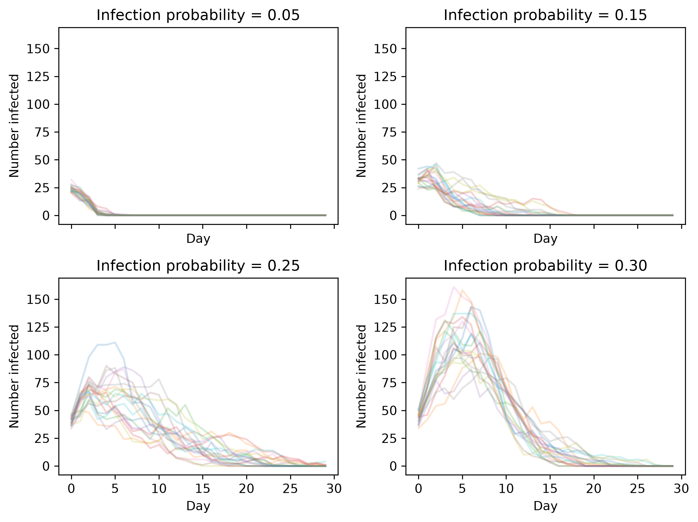
Figure 6.1: Epidemic trajectories across four processes without migration

So far we have side-stepped the question of migration. The remainder of the chapter tackles that topic.

6.2 Manager, Barrier, and Shared Data Structures

We now want to allow for inter-process communication. This will open the door for migration in our epidemic code. Data sharing across processes is facilitated by Python’s multiprocessing.Manager class that creates a standalone server process to hold and manage centralized Python objects. It provides the means to safely share complex objects like lists and dictionaries. The listing below illustrates using a shared dictionary and how things can sometimes go wrong.

from multiprocessing import Manager
from multiprocessing.pool import Pool
import time

def worker(worker_id, mailboxes, barrier):

    if worker_id == 0:
        mailboxes[1][:] = [2, 3, 7]
        
    # wait until all workers reach this point
    # barrier.wait()
   
    if worker_id == 1:
        mailboxes[2][:] = mailboxes[1][:]
    if worker_id == 2:
        mailboxes[0].append(200)

    return

def mailbox_demo():

    # create a manager to tend to shared memory objects
    with Manager() as manager:

        # shared dictionary with one mailbox per worker
        mailboxes = manager.dict({
            0: manager.list(),
            1: manager.list(),
            2: manager.list()
        })

        # shared barrier
        barrier = manager.Barrier(3)

        # information to be sent to each process 
        set_up = [
            [0, mailboxes, barrier],
            [1, mailboxes, barrier],
            [2, mailboxes, barrier]
        ]

        # create the pool and send information to the workers
        with Pool(processes = 3) as pool:
            pool.starmap(worker, set_up)

        final_mailboxes = {k: list(v) for k, v in mailboxes.items()}

    return final_mailboxes

# Protect against multiple pool creations
if __name__ == "__main__":
    print(mailbox_demo())

The listing creates a shared dictionary object for three worker processes. Recall, that a dictionary is a data structure composed of (key, value) pairs. In this instance, the keys are the process identification numbers, either 0, 1 or 2, and the value or data components are lists. There is also a shared barrier object whose purpose is to synchronize writing and reading operations. Both the shared dictionary and barrier objects are created in the calling program mailbox_demo, bundled into a set_up list and sent to the worker function via starmap. On return to mailbox_demo the dictionary comprehension for final_mailboxes creates an ordinary (not shared) dictionary whose values are ordinary (not shared) lists that persist after the manager is shut down. items() is a dictionary method. It returns the dictionary’s key-value pairs.

Once we enter the worker function, process 0 writes to the process 1 list and then process 1 assigns the process 1 mailbox contents to process 2. Process 2 merely appends 200 to the data for process 0. The output from the program should look like

[[200], [2, 3, 7], [2, 3, 7]]

But, results such as

[[200], [2, 3, 7], []]

happen on occasion. The problem here is that the processes are working independently and sometimes process 1 reaches its if statement before worker 0 has had a chance to write its data leaving mailbox[2] with an empty list. This is a classic example of a race condition. A mix-up occurs because worker 1 uses mailboxes[1] before worker 0 has finished writing to it. The problem goes away if we uncomment the barrier.wait() line. The barrier forces all workers to pause until every worker has reached the synchronization point. Since worker 0 performs its write before the barrier, worker 1 cannot proceed to the copy operation until that write has completed. This was an easy problem to fix; but, we must be aware that synchronization is necessary to avoid race condition errors and race conditions are not always so easy to detect as in this example.

6.3 SIRD: Migration

Using what we learned from the mailbox example in the previous section, we are ready to deal with incorporating migration into our epidemic code. The idea is that now n_migrants per day will move from one town to another. For simplicity this will be accomplished via a round-robin strategy wherein n_migrants move from town 1 to town 2, from town 2 to town 3, from town 3 to town 4 and finally from town 4 back to town 1, closing the loop. This choice of how individuals migrate is simply for coding convenience and not intended to model any real-world mechanism. The immigrants will be randomly chosen from the “town’s” population and new arrivals will be appended to the end.

Conceptually, adding migration to the epidemic mix requires little more than adding another function call to worker: one that carries out the migration step. A pseudo code description of this function is

As seen in the mailbox example of Section 6.2 transferring migrants and synchronizing processes requires barriers and shared data structures. The way to do this is with multiprocessing.Manager and we need to integrate this into our code somewhere. The most natural spot is sim_template and a modified version of that program that has the new features we need is

from numpy.random import default_rng, SeedSequence
from multiprocessing import Pool, Manager
from epidemic_worker import worker 

def sim_template(seed, n, n_reps, n_cores, *args):

    ss = SeedSequence(seed)
    child_seeds = ss.spawn(n_cores)

    rg_list = [(default_rng(s), i) for i, s in enumerate(child_seeds)]

    with Manager() as manager:

        barrier = manager.Barrier(n_cores)

        mailboxes = manager.dict()
        for i in range(n_cores):
            mailboxes[i] = manager.list()

        set_up = [[0] * 6 for _ in range(n_cores)]

        for i in range(n_cores):
            set_up[i][0] = rg_list[i]
            set_up[i][1] = n
            set_up[i][2] = n_reps
            set_up[i][3] = barrier
            set_up[i][4] = mailboxes
            set_up[i][5] = args

        with Pool(processes = n_cores) as pool:
            result = pool.starmap(worker, set_up)

    return result

There are three primary differences between this sim_template and the canonical version in Chapter 4. First, the set_up list has two additional components: barrier and mailboxes: a barrier object and shared dictionary as in the mailbox example. Secondly, it uses the tuple version of rg_list presented earlier that furnishes each core with a numeric identifier. The parameter n_reps is now constant across cores and load balancing is no longer necessary. That aspect of the old sim_template has been omitted. There is also another, hidden, difference in the migration version of sim_template. The parameter n_migrants we have heretofore ignored will come into play.

Following the pseudo-code outline a Python version of the migration function takes the form

def migration(rg, population, recovery_time, death_day, n_migrants,
              worker_id, n_cores, barrier, mailboxes):

    if n_migrants == 0:
        return

    n_send = min(n_migrants, len(population))
    dest = (worker_id + 1) % n_cores

    for _ in range(n_send):

        migrant = rg.integers(len(population))

        mailboxes[dest].append([
            population[migrant],
            recovery_time[migrant],
            death_day[migrant]
        ])

        population.pop(migrant)
        recovery_time.pop(migrant)
        death_day.pop(migrant)

    barrier.wait()

    for person in mailboxes[worker_id]:

        population.append(person[0])
        recovery_time.append(person[1])
        death_day.append(person[2])

    # empty the mailbox
    mailboxes[worker_id][:] = []

    barrier.wait()

Here n_send is the number of migrants to be sent by each process and dest is where the process will send them. Each process pops n_send random subjects and places their data in the receiving process’ mailbox. After that there is a pause until all processes complete the sending phase. Then, each process receives the migrant information that has been placed in its mailbox and incorporates it into its population. Everyone waits until all workers have finished the receiving phase, I_history is returned to the master process and the worker has finished its task.

To put these pieces together the worker of Section 6.1 needs only two small changes, which is why we do not reprint the whole function here. First, its signature grows to worker(rg_and_id, n, n_reps, barrier, mailboxes, param_tuple) so that it can receive the barrier and shared mailboxes that now travel in each six-element set_up list. Second, inside its daily loop, just after the infection updates, it adds the single call migration(rg, population, recovery_time, death_day, n_migrants, worker_id, n_cores, barrier, mailboxes). The worker_id, n_migrants, and n_cores it passes along are already on hand: worker_id came unpacked from rg_and_id, and n_migrants and n_cores from param_tuple, exactly as before. Everything else is unchanged, so each simulated day now ends with n_migrants individuals hopping to the next town while the shared barrier keeps every process’ send and receive operations in lockstep.

Figure 6.2 illustrates the consequences of migration. The round-robin strategy has the effect of mixing less infectious subjects into the populations for processes 2-4 and more infectious subjects into the population for process 1. Comparing with Figure 6.1 migration appears to add to variability and prolong the epidemic’s life.

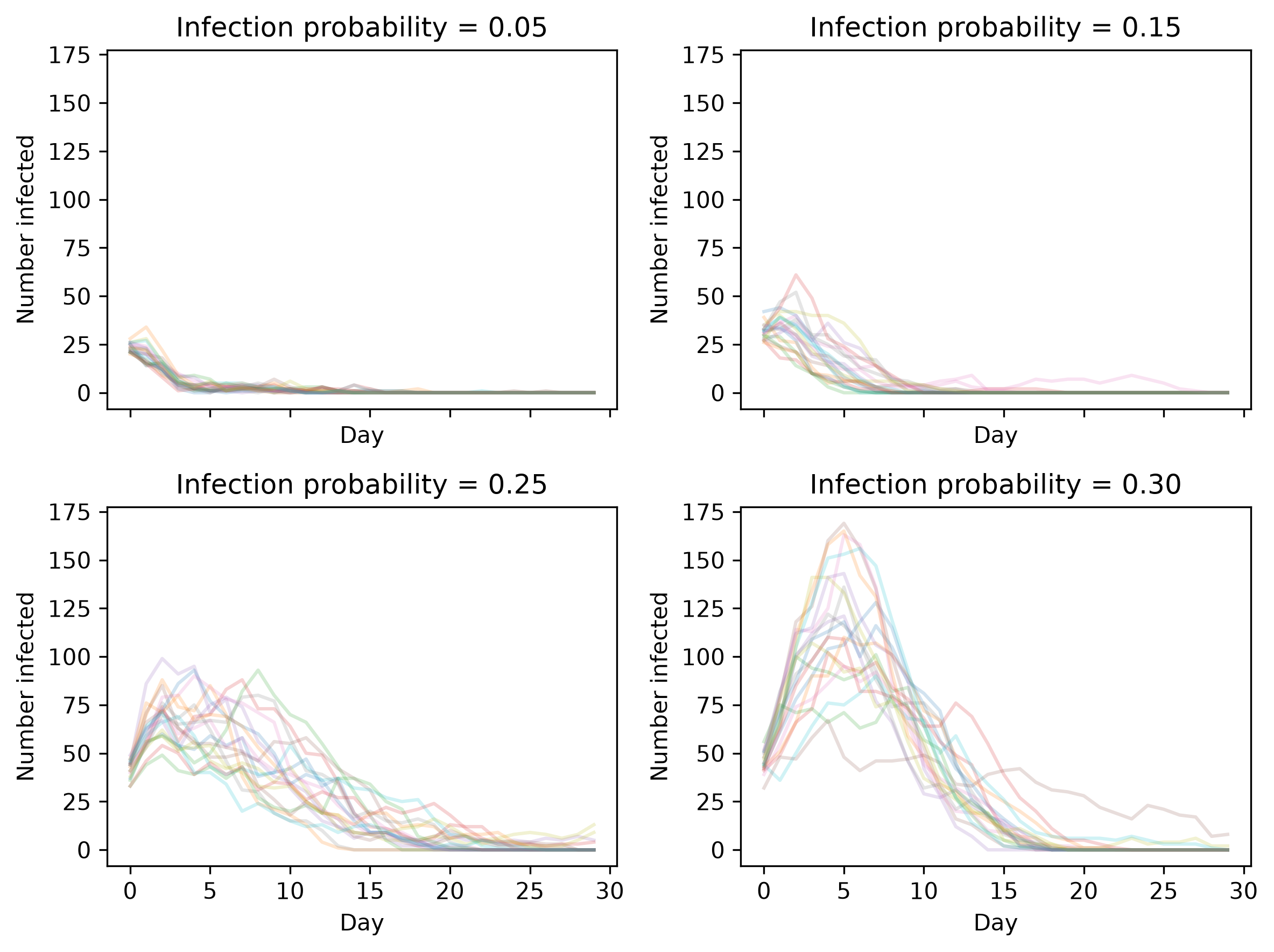
Figure 6.2: Epidemic trajectories across four processes with migration

The migration mechanism transformed the problem from a collection of independent stochastic simulations into a single interacting system. Even though each process is governed by its own transmission probability, the exchange of individuals allows infection to propagate between populations, producing dynamics that differ qualitatively from the independent case. In particular, populations with higher transmission rates tend to export infection, while those with lower rates import it, leading to a more homogeneous overall pattern. This illustrates how parallel computation can be used not only to accelerate simulation, but also to model interaction and dependence across components of a system. In this way, parallel simulation becomes a tool for modeling complex systems, rather than simply a means of reducing computation time.

The Manager and Barrier objects we relied on here are only two of the tools Python’s multiprocessing module offers for coordinating processes that share states. A Lock enforces mutual exclusion, letting just one process touch a shared resource at a time, which is a direct cure for the race condition we saw earlier. A Queue passes data between processes in a safe, orderly way, so one process can hand results to another without their writes colliding. A Barrier, the tool we chose, holds every process at a checkpoint until all have arrived, keeping the day-by-day clock in step. Migration is just one application of shared states. Whenever cores must coordinate rather than run in isolation, the right primitive depends on what they need: to take turns (a Lock), to exchange data (a Queue), or to advance in lockstep (a Barrier).

6.4 Chapter Summary

In this chapter, we extended our basic sim_template code to incorporate a SIRD epidemic model. This furnishes a means to study the mechanics of disease progression in a virtual environment that resembles what may transpire in the real world. By thinking of the processes as representing towns it became possible to introduce migration into the epidemic framework. This required us to use tools for inter-process communication such as Manager objects for shared memory supervision, barrier objects, and shared data structures. We saw that the introduction of inter-process communication appreciably changed the infection trajectories from the no-migration case.

Chapters 3 through 6 have walked us through our basic simulation framework along with two case studies. The next chapter, Chapter 7, steps back to the operational details. We address questions such as how do you count cores correctly on your machine? What happens when memory becomes the bottleneck? How do you detect and stop runaway worker processes, and benchmark parallel code properly?