2 Random Numbers and Simulation

Chapter 1 framed the goal. We need to investigate the properties of a statistical measure under repeated sampling. In practice that means running repeated experiments in a controlled environment. The modern venue for such a study is simulation on a computer: the data scientist’s laboratory.

2.1 What is a Simulation?

If you have acquired a copy of this book it is very likely that you have an idea of what the term simulation means. But, it is worthwhile to give it a precise meaning here. In particular, it is useful to clarify the difference between the general definition and the connotation we will use in the book.

A simulation is an imitation of a real-world process. It can be a physical event; but, our focus is on virtual, statistical simulations that are carried out on a computer. In that context a simulation is merely this: you build an artificial data set under conditions you control, you compute the number (or numbers) you care about, and you repeat that many times. Each new data set represents an experiment and in combination they comprise a simulation experiment.

The conditions you control are the (assumed) probability framework that models the collection of data in some real world setting. The numbers you compute are statistics: quantitative information computed using only the (simulated) data values such as summary measures like the average, confidence intervals, and test statistics. If you can describe how your data are generated and write down the number you want from them, you can run a simulation experiment.

Why repeat? Because any single data set is but a single draw from a random process and the numbers you compute from it are therefore also random. This means they are subject to random variation. If you run the experiment once you will learn very little; the value you obtained could have been noticeably higher or lower purely by chance. On the other hand, if you run it hundreds or thousands of times patterns will emerge to reveal what can be expected in a general sense and this will tell you how much trust to place in the value of your statistic.

Repeated simulation follows the same logic a lab scientist uses when they run an experiment many times rather than once. The difference is that here the laboratory is the computer and a single trial costs microseconds instead of weeks. That cheapness offers an opportunity. It lets us ask “what would happen if…” and get an answer by brute repetition instead of possibly intractable mathematical finesse. The one cost you cannot escape is the repetition itself. Serious answers usually need hundreds or thousands of repeated samples, which can be a lengthy endeavor if the samples are generated and processed one at a time. But, speeding up many repetitions of a slow computation is exactly the problem the rest of this book sets out to solve.

The output from a simulation study is a cloud of statistics that you study to assess patterns that reflect on the performance of your procedure. How wide is the cloud? If your statistic is a point estimator is the cloud centered at the parameter value specified in the model or are the estimates systematically off-target? Do the statistics behave badly with heavy tails or a small sample size? If you are looking at a test statistic does the cloud conform to the proper null distribution and does it show power against an alternative? Each question becomes a what-if experiment.

It helps to place names on the characteristics of the cloud of simulated values. For a point estimator its center, compared to the true parameter value in the model, is bias: is the estimator systematically high or low? Its width is variability: how much would the answer change for a new data set? If the statistical procedure produces a confidence interval or test statistic, you count how often that interval contains the true value or the test rejects the null model when it is false. Bias is being off-target on average; variability is the scatter of the generated numbers; coverage is how often your stated (confidence) net actually catches the numerical “fish”; power is the proportion of times your test rejects a false model.

The driving force behind any computer simulation experiment is its random number generator that produces the data. This suggests we should explore that subject before going further. Appendix B and C provide some directed discussion of the topic. The next section gives a high level discussion of random number generation that will set the stage for the work that follows.

2.2 What is a Random Number Generator?

In its simplest form, a random number generator is a numerical algorithm that is designed to produce a stream of numbers that behaves like a random sample from the uniform distribution. Random number generators have myriad practical applications in areas like digital security, computer gaming, sampling, gambling and lotteries, and artificial intelligence. Our interest here is in using them for statistical simulation.

Despite their name, random number generators are deterministic. The generated numbers depend on a value (or values) called the seed. Assuming it is implemented correctly, the sequence of values you produce with a random number generator is completely determined by the choice of the seed. That is, given an identical seed, you’ll always replay the identical “random” sequence, making your simulations fully reproducible. Consequently, this kind of generation is usually called pseudorandom rather than random. We’ll often use the term “random” going forward; but, keep in mind that it’s really pseudorandom.

Although random number generators cannot produce truly random values, the numbers can appear random and pass statistical tests for randomness. That is, in fact, how generators are evaluated and there are suites of tests developed solely for that purpose. The classic example of such a suite is the Diehard tests developed by George Marsaglia. A more recent test battery is TestU01 from L’Ecuyer and Simard (2007) and we take it to be the modern standard for evaluating a generator. TestU01 contains three batteries of tests: Small Crush, Crush, and Big Crush which contain 10, 96, and 106 tests, respectively.

Of course, we need to be able to simulate from probability distributions other than the uniform. Fortunately, that is not difficult.

Every probability distribution has a quantile or percentile function \(Q\). The value of \(Q(p)\) is the \(p\)th percentile of the distribution. In particular, \(Q(.25), Q(.5)\), and \(Q(.75)\) are the first quartile, median, and third quartile, respectively.

A key feature of the quantile function is that, if \(U\) is uniformly distributed on \([0, 1]\), \(Q(U)\) has the same distribution as the random variable \(X\) with quantile function \(Q\). So, suppose we have a target probability distribution in mind. To obtain a random sample from that statistical model we can proceed as follows.

An illustration of the algorithm at work is provided by Figure 2.1. There are two histograms in the figure. The top one corresponds to a random sample of 100,000 uniform random variables. The bottom one is the same sample after transformation using R’s standard normal quantile function qnorm. The transformed data is therefore a pseudo-random sample from the standard normal distribution. The histogram certainly exhibits the characteristics we would expect from a normal random sample and goodness-of-fit tests do not reject that hypothesis. We use this algorithm again in Chapters 3 and 4.

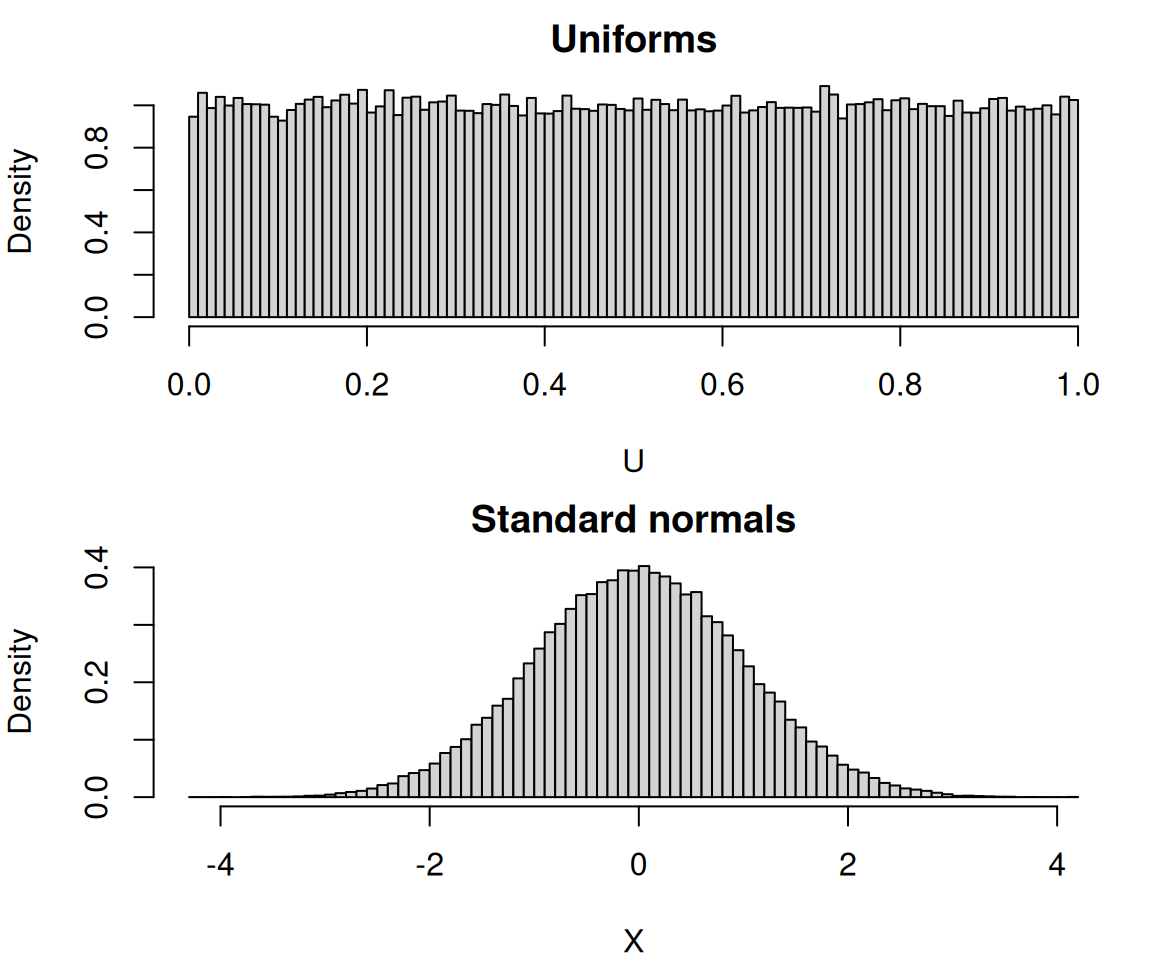
Figure 2.1: Uniform and normal histograms.

2.3 Accessible Warm-Up Examples

Three small problems place the idea of simulation experiments in familiar settings. The first of them, estimating \(\pi\), comes back later as real, parallelized code in Chapters 3 and 4. The birthday and power problems stay here as warm-ups.

Estimating pi by throwing darts. Picture a square dartboard two units on a side, centered at the origin, with a circle of radius one drawn inside it that just touches the edges. The square has area 4 (that is 2 times 2). The circle has area \(\pi\). So, if you experiment and throw darts in such a way that each dart is equally likely to land anywhere in the square, the long-run fraction landing inside the circle is the ratio of the two areas, \(\pi / 4\). Multiply the observed proportion of darts falling in the circle by 4 and you have an estimate of \(\pi\).

We can simulate the physical dart game experiments with a random number generator on a computer. Our basic experiment is to throw n darts which returns an estimator of \(\pi\). Then, we repeat this n_reps times to explore how the estimator works in repeated samples. The resulting pseudo-code algorithm looks like

It is worth reading this listing one line at a time, because most of the examples in the book have this same shape. The steps are:

• Set the random seed to fix the starting point of the random number generator so the whole experiment can be reproduced exactly later.

• Start with hits set to 0 and use it to keep a running tally of virtual darts that land in the circle.

• Throwing the dart n times is the experiment: each pass through the loop is one virtual dart thrown and one independent trial.

• In the interior loop the two uniform random numbers in \([-1, 1]\) locate the dart: a uniform draw means every position in that interval is equally likely, and using the interval from -1 to 1 for both \(x\) and \(y\) coordinates makes the dart land anywhere in the 2-by-2 square with equal chance.

• The logical if test asks whether the dart is inside the unit circle, because a point is in the circle when its distance from the origin is at most 1.

• When the test returns true we add one to hits so that, after the inside loop, the ratio of hits to n is the fraction of darts landing in the circle. Average the ones (in) and zeros (out) and multiply by 4 to have an estimate of \(\pi\).

• The outer loop represents repeats of the basic experiment. It returns a vector of n_reps \(\pi\) estimates that can be combined for a composite estimator and/or further analyzed to gain insight into the estimator’s sampling distribution.

Because the estimator is an average of zeros and ones, its accuracy improves the way averages do: the error shrinks roughly like one divided by the square root of the number of darts or n. That square-root law is worth internalizing because it governs almost every Monte Carlo estimate you will ever compute. It means accuracy is expensive. To halve the error you must quadruple the work. A few thousand darts pin down only the first digit or two of pi, and getting a couple more digits reliably takes on the order of a million throws. Slow convergence like this is precisely why we need a way to speed up the computation.

The birthday problem. How many people must be in a room before two of them share a birthday more often than not? Most people guess a number near 183, half of 365. The answer is 23, and the reason is worth the detour.

What matters is not so much the number of people but rather the number of pairs, because each pair is a separate chance for a match. A room of 23 already contains 253 pairs (23 times 22 divided by 2) and a collision becomes likely far sooner than intuition expects. You can derive the exact probability; but, you can also simulate it, which doubles as a check on the accuracy of the derivation.

This skeleton code is almost identical to the dartboard example. Only the middle section changes. Dissecting this line by line produces

• Draw room_size birthdays, each uniformly distributed on the integers from 1 to 365, to fill a virtual room. Each virtual person gets a day of the year chosen uniformly, ignoring leap years and the small real-world bumps in the birth calendar, both of which barely move the answer.

• Determining if any two birthdays are equal again produces yes-or-no outcomes for the room;

• Each coincident birthday adds one to matches, and at the end the matches to n_reps fraction is the estimated probability of a shared birthday for that room size.

• Run this experiment to estimate the probability of a birthday match for a given room size. Then repeat the same basic experiment across a range of room sizes and you will see the curve rise steeply, passing one half at 23 people in the room and exceeding 99% by about 57.

Will the experiment even detect the effect? This third example is closer to day-to-day data science. Before running an A/B test or a small study, you would like to know whether it has a decent chance of finding a real effect of the size you care about.

You have a control or null model in hand and a variant or alternative in mind. The question is then one of statistical power and there are formulas for that only in the simplest cases. On the other hand, it is a one-paragraph simulation in any design, viz.

Again the code has the same skeleton. The data-generating step bakes in the effect size you want to be able to catch at the sample size you can afford. The “quantity of interest” is just whether your usual test, run exactly the way you would run it on real data, comes back significant. Averaging those yes-or-no outcomes over many simulated data sets estimates the probability the real study will be worthwhile. If the estimated power comes back at 0.45, say, you have learned (cheaply!) before collecting a single real observation, that the planned study is roughly a coin flip and the sample size needs to grow.

All three warm-up examples exhibit the same loop: generate something random, reduce it to a single number, and average over many repetitions. Everything else in this book is a more elaborate version of that loop. Thus, it is worth stating the general theme once, in plain language, before any code appears:

2.4 Simulating in Parallel

One way to reduce the time it takes to run many physical experiments is to spread them out across multiple workers. In the case of a physical laboratory, for instance, several experiments can be performed simultaneously by different technicians. For experiments on a computer, the role of a technician is played by a virtual worker process running on one of the machine’s processors. Farming the work out across cores is one instance of parallel processing.

This basic divide-and-conquer strategy is fine in principle. But, in the laboratory context care must be taken to ensure that the technicians do not collaborate and work independently. Similarly, the individual processes on the computer need to produce independent random number streams to ensure they do not duplicate each others’ efforts. An extreme case occurs when the same generators are used for each worker with the same seed. In that instance the results returned by every processor are exactly the same. This is like technicians copying each other’s reports.

Somewhat more realistic is the instance where two different seeds may simply place the generators at different points on the same cycle. The resulting streams are not independent but rather are shifted copies of one another. The technicians/processors share information and do not produce identical results; but, their outputs remain deterministically linked.

A generalization of the previous serial simulation algorithm now takes the following form

Each step in the algorithm earns its place. The first step is to record a single number that can be used to regenerate the entire experiment exactly; without it, a surprising result cannot be reproduced or debugged, and “I cannot reproduce the number from last week” is a far worse problem in a study than in ordinary software.

The next step is the subtle one that is easy to get wrong. A generator has only one built-in sequence; a seed does not create a new sequence, it only chooses where you start on that particular sequence. So the tempting shortcut, give worker 1 seed 1, worker 2 seed 2, and so on, does not hand the workers independent streams. It hands them the same sequence read from different starting points, with no guarantee those points are far apart. If they are close, or if each worker draws enough numbers, they begin reusing each other’s values; and even when they never overlap, one worker’s stream is just another’s shifted along the same fixed list. In either case the draws are deterministically linked rather than independent and several workers quietly do related work. The presence of the extra workers buys you confidence you have not actually earned. Nor is the problem easy to catch: streams with strong built-in dependence can pass every test in the standard batteries (Ismay 2013).

Throughout this book we use the PCG64 generator developed by O’Neill (2014). It produces a very large number of independent streams that parallel code can access easily, and it passes the modern statistical-test batteries. It is available in R through the dqrng package, and it is Python’s default generator. Appendix C covers how PCG64 works internally. Appendix B sketches alternatives for readers who want to compare PCG64 with other viable parallel options like MRG32k3a, Threefry, and Philox.

The third step is load balancing: the n_reps repetitions are split among the workers so that they finish at about the same time, which is what actually shortens the wall-clock execution time. It is rarely as simple as n_reps divided by the number of workers; a million-and-three repetitions over eight workers, for example, cannot be split evenly. So, the leftovers have to be prorated in a way that balances the computational effort.

The fourth step is the only part that changes from problem to problem. It is where data is generated and the estimator is computed. It is the code you actually write.

The final step is to combine the per-worker results. Usually this is accomplished by pooling or averaging.

The answer produced by this parallel Algorithm is identical in expectation to the single-worker version treated earlier. But, it arrives at its destination sooner depending on how many workers are involved. The only piece specific to \(\pi\) estimation or the birthday problem or the power loop from the previous section is the data generation and estimation step. All the other steps remain the same.

That is the practical payoff of stating the algorithm this way. Since all but one of the basic steps barely change from one problem to the next, they can be written once, as a reusable template, leaving you to supply only the step that is problem specific. That template is our somewhat generic program sim_template presented in subsequent chapters. Its call will take the seed, the per-replication sample sizes (n), the number of replications (n_reps), the number of workers (n_cores), and any model parameters, which is simply the pseudo-code recipe given a function signature. Chapters 3 and 4 build it in R and Python, and Chapters 5 and 6 show it carrying real research problems with only the worker being swapped out.

2.5 A Caveat

Everything in this chapter relies on a fundamental premise: the “uniform random numbers” we draw actually behave randomly. That need not be true and the failure to satisfy that condition can be hard to diagnose. An illustration of how it can go wrong is provided by the tale of the generator RANDU discussed in more detail in Appendix B. It shipped on widely used mainframes through the 1960s and 1970s. RANDU’s parameters produce streams satisfying an exact linear relationship between consecutive triples having the consequence that every single point lies on one of just fifteen parallel planes, a stack of thin sheets with wide empty gaps between them. That defect was not academic. For years, Monte Carlo studies built on RANDU produced results that were quietly wrong, and wrong in a way nobody caught because the numbers still passed the simple one-dimensional checks people typically applied.

It is hard to overstate the gravity of this error. Any simulation that effectively groups the stream into triples, and many do without anyone noticing, samples from those fifteen planes instead of from the cube. Thus, an integral comes out biased or a variance comes out too small; the reported uncertainty is confidently wrong.

The general lesson outlasts the specific generator: looking random in one dimension is not the same as being random and damaging correlations can lurk in higher dimensions where no one is looking. This is why serious generators are now vetted against demanding test batteries: the Diehard tests and especially TestU01 from L’Ecuyer and Simard (2007), whose Small Crush, Crush, and Big Crush suites probe exactly these higher-dimensional structures. It is also why this book standardizes on the PCG64 random number generator rather than whatever a language happens to ship by default.

2.6 Chapter Summary

In this chapter we gave a big picture discussion of generating random number streams in both serial and parallel code. The importance of both between and within stream randomness was highlighted.

The fundamental quantile transformation was explained in Section 2.2. This tool allows us to simulate from any probability distribution if we have a uniform random number generator.

Several examples of simulation experiments were described that all follow a similar pattern. This feature makes them amenable to treatment from the template perspective of Chapters 3 and 4.

In the next chapter we get specific and turn to running simulations in parallel in R. Let us begin.