5 Case Study: Segmented Regression with Bootstrapping in R

The parameter estimation problems in Chapter 3 were deliberately lightweight. Nonetheless, they illustrated the central idea we have built on here: compute your estimator from data obtained from some specified model, then draw a fresh data set and compute it again, over and over. The resulting estimator values when taken all together provide an empirical assessment of the sampling distribution of the estimator. It is that distribution that tells us how much trust to place in any single estimate. The Cauchy example was a rudimentary but thorough illustration of how simulation can approximate the sampling distribution for a parameter estimator.

In general, however, both the modelling and estimation phases of sim_worker will be much more involved than what we saw in Chapter 3. In particular, parameter estimation typically requires optimization of some performance criterion. With that in mind we now expand our horizons and demonstrate how sim_template can be used effectively to obtain information about the sampling distributions of point and interval estimators in a more demanding environment.

5.1 Problem Setting and Data Generation

Suppose we can assume there is a linear relationship between a response and an independent variable. But, unlike simple linear regression, the model is segmented. There is one regression line that applies up to a point $\theta$, then there is a jump and a different line takes over on the other side. Figure 5.1 shows a picture of the general idea.

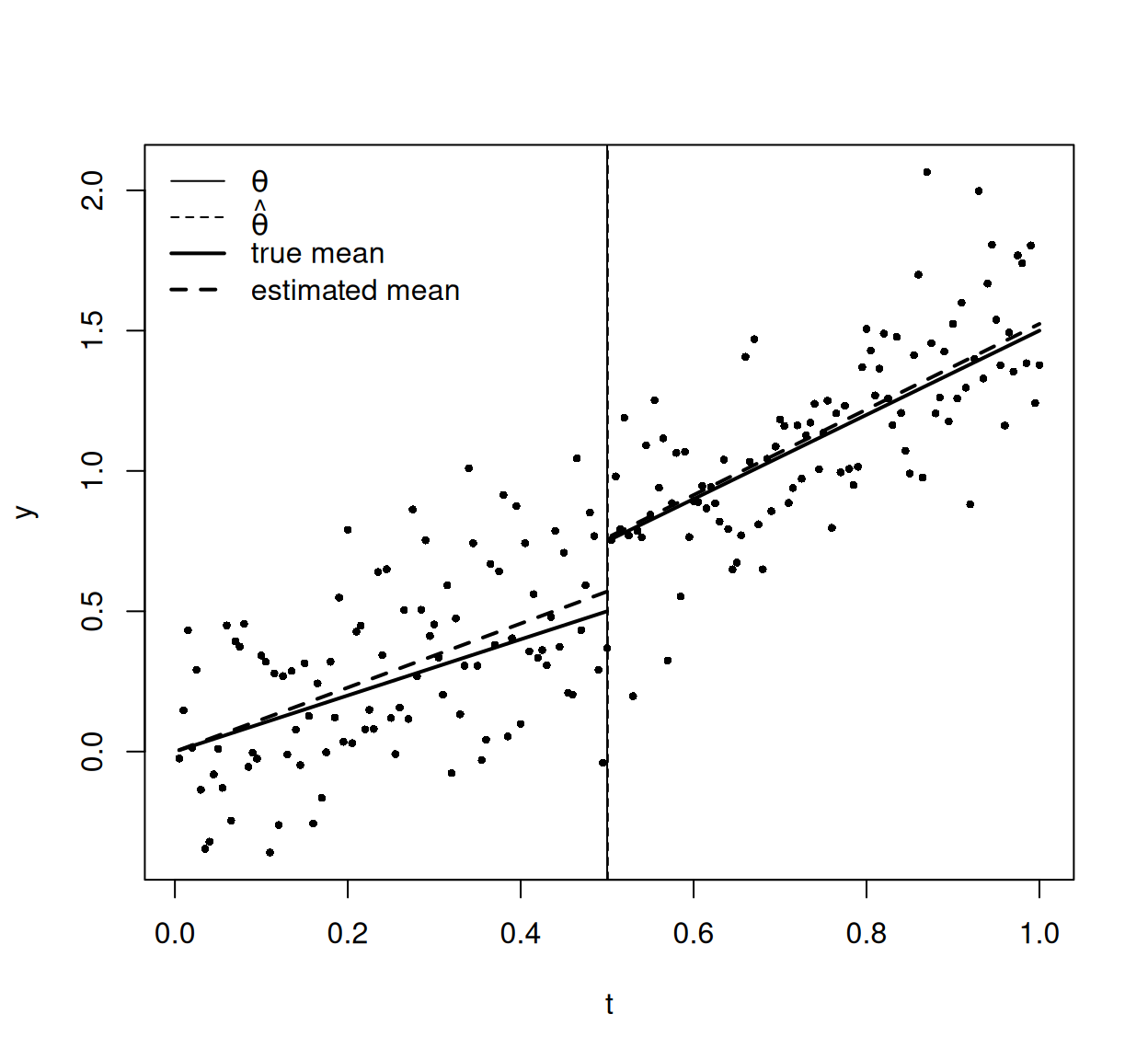
$Change-point Data. At this scale the vertical lines for $\theta$ and $\hat\theta$ overlap almost completely.$

Figure 5.1: Change-point Data. At this scale the vertical lines for $\theta$ and $\hat\theta$ overlap almost completely.

There is a lot going on in Figure 5.1. But, focus your attention on the solid curve that represents the population mean function. Here we see random scatter around a broken line with a discontinuity at $\theta$ = .5. Models like this arise in a variety of contexts. For example, in Economics changes in regulations or tariffs can produce sharp changes in regression regimes. Simulating from such models facilitates forecasting the progression of interest rates, economic indicators, etc.

To make life simple we will assume normal random disturbances or errors for our regression model with some associated, unknown, standard deviation. The code listing below will produce data from such a model given choices for its parameters.

dat_gen <- function(n, theta, beta_1, beta_2, sigma){

  # set the seed for R's random number generator
  set.seed(1234)
  
  # install and seed the PCG64 random number generator
  library(dqrng)
  dqRNGkind("pcg64")
  dqset.seed(generateSeedVectors(1)[[1]], generateSeedVectors(1)[[1]]) 

  # array of normals with standard deviation sigma
  epsilon <- dqrnorm(n, mean = 0, sd = sigma)
  
  # uniformly spaced predictor variable
  t <- 1:n/n
  
  # response vector with slopes beta_1, beta_2 and change point theta
  y <- beta_1*t*(t <= theta) + beta_2*t*(t > theta) + epsilon
  return(list(t = t, y = y))
}

The beginning of the listing follows the now familiar pattern of invoking the PCG64 generator from the dqrng package and then setting its seed and increment with the generateSeedVectors function. The next step is to generate the vector of normal random errors. That is accomplished with the dqrnorm function from the dqrng library. The way we have done it by first specifying dqRNGkind("pcg64") means that the bit sequence produced by PCG64 will be used along with a fast algorithm to produce pseudo-random normal deviates with standard deviation sigma. The independent streams aspect of PCG64 therefore carries over to the sequences of random normals.

The independent variable in the model, t, is composed of n uniformly spaced points in the interval $[0, 1]$ with n the sample size. This vector of values is translated into two “predictor” variables: t*(t <= theta) and t*(t > theta). These are products of t with vectors of TRUE/FALSE values indicating the location of the elements of t relative to theta. The logical constants assume values of 1 and 0 in the products to create the piecewise linear regression curve.

By choosing sigma = .25, beta_1 = 1, beta_2 = 1.5 and theta = .5 in dat_gen we arrive at the data in Figure 5.1.

5.2 Model Fitting

The goal of all this is estimation of $\theta$. But, there are other parameters that must also be estimated. The trick for doing that is to observe that suitable values for beta_1, beta_2 and sigma can be calculated directly given any specific choice for $\theta$. Code that does this for the coefficients looks like

fit_theta <- function(theta, t, y){
  
  # design matrix
  X_theta <- cbind(t*(t <= theta), t*(t > theta))
  
  # least-squares fit
  lm.fit(X_theta, y)
}

This creates the design matrix X_theta of “predictor” variables and then uses lm.fit to estimate the regression coefficients conditional on the value of theta used in X_theta. The lm.fit function is a computationally efficient alternative to the model based lm function. This is important when fitting many regressions like we will here.

The lm.fit function returns several fit related quantities including fitted.values and coefficients as well as residuals. For example, in the case of theta = 0.5008354 the fitted coefficients for the two line segments and the standard deviation estimator are found to be

n <- 200
out <- dat_gen(n, .5, 1, 1.5, .25)
t <- out$t
y <- out$y
reg_fit <- fit_theta(0.5008354, t, y)
sig_hat <- sqrt(sum(reg_fit$residuals^2)/n)
c(reg_fit$coefficients, sig_hat)

##        x1        x2           
## 1.1406857 1.5239528 0.2527598

These correspond to the estimated mean curve in Figure 5.1. The estimated values can be compared to 1, 1.5 and .25 which were the true values that produced the data.

But, why use this particular choice for theta? That question leads us into the problem of how to estimate $\theta$.

We have seen that for any given $\theta$ we can compute the least-squares fit to the data. But, which of all these possible fits should we choose. An intuitive response is to say “select the one that best fits the data.” Of course that begs the question of what you mean by best. For our purposes we will define “best” as the estimator $\hat\theta$ of $\theta$ that minimizes the residual sum-of-squares

SSE <- function(theta, t, y){
  sum(fit_theta(theta, t, y)$residuals^2)
}

Using this function we find

SSE(.5, t, y)

## [1] 12.7775

SSE(0.5008354, t, y)

## [1] 12.7775

So, this mysterious value 0.5008354 for theta fits the data exactly as well as the true value of the change point parameter. That is no accident: none of the observed t values fall between .5 and 0.5008354, so the two choices produce the same design matrix and hence the same least-squares fit. In fact, if we were to search over all of the unit interval we would find that no break point does better. The value 0.5008354 attains the global minimum of the residual sum-of-squares and that is how we plan to find our estimator $\hat\theta$ of $\theta$ in general.

The question now becomes one of optimization of the residual sum-of-squares criterion. A plot of that function for our example data set is shown in Figure 5.2. It has several peaks and valleys which would pose problems for most minimization algorithms, which typically assume a simple bowl-like shape for the function being minimized. Of course, if you start at the right location a local bowl shape can often be expected.

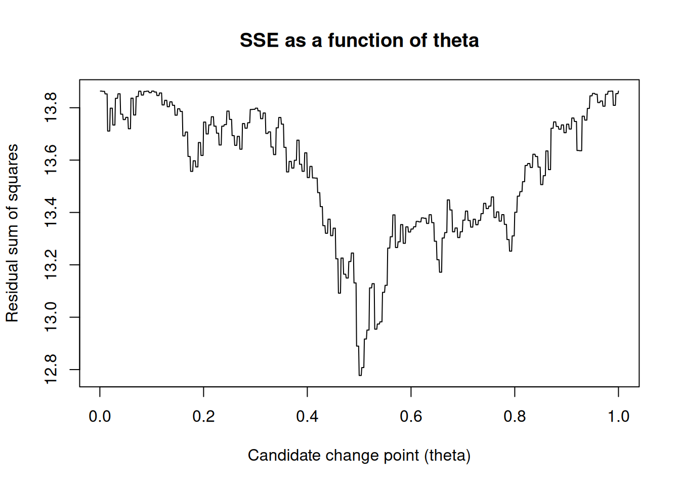
Figure 5.2: Residual Sum of Squares

The key then is to find the right starting point. For that purpose one can use a global random search. For instance, use a uniform random number generator to scatter points over the interval $[0, 1]$, evaluate the SSE criterion at each of them and retain the one that returns the smallest value. Code that accomplishes this with 100 search points takes the form:

trial_values <- dqrunif(100)

# compute SSE for each trial value
sse_vals <- sapply(trial_values, function(x) SSE(x, t = t, y = y))

# find the minimizer of sse_vals
theta_start <- trial_values[which.min(sse_vals)]

For our example data set we find theta_start = 0.5009544. The next step is to combine this good starting point with a numerical minimization procedure. For that purpose we choose Brent’s method from R’s optim function.

Since we know $\theta$ is in the interval $[0, 1]$ we can take lower = 0 and upper = 1 for those Brent parameters. Combining this with our rough estimator theta_start as a starting or initial evaluation point gives

theta_hat <- optim(theta_start, SSE, y = y, t = t,
                   method = "Brent", lower = 0, upper = 1)$par

which produces $\hat{\theta}$ = 0.5008354 as an estimator of the slope change point and solves the mystery.

So, now we have a method for estimating $\theta$. How can we expect this approach to work in practice?

Some answers exist in the statistics literature. Bai (1996) shows that $\hat\theta$ converges to the true change point in a probabilistic sense as the sample size grows large. But, the standard textbook recipe for a confidence interval does not apply here. For a 95% interval that recipe pretends that $\hat\theta$ is approximately normal for large n, then adds and subtracts two standard errors. Among other things this formulation assumes that the regression function is smooth in $\theta$, and ours has a discontinuity. So, we need an alternative approach such as the bootstrap which may or may not be effective.

This places us in new territory. The Cauchy and $\pi$ estimation examples of the previous two chapters used simulation in a confirmatory capacity. The theoretical (e.g., large sample) properties of the estimators were known and the simulation investigated how well they held in practice. In contrast, for the segmented regression problem, the available theory is rather sparse moving our purpose to one of exploration rather than confirmation. We are not attempting to establish general theoretical properties of the estimator. Instead, we will use simulation to identify features that appear promising, diagnose potential problems, and formulate questions for further study. Specific issues to be addressed are

Does the point estimator appear centered near the true change point?
Does its sampling distribution resemble a normal distribution?
Do the bootstrap confidence intervals attain their nominal coverage levels?

5.3 Bootstrapping and Interval Estimation

To this point we have studied an estimator by simulating from a model whose parameters we specify at the outset. For a real physical experiment the parameters are generally unknown and we cannot generate fresh data at will. The bootstrap is a clever way around this seeming impasse. It treats the single data set you actually collected as a stand-in for the population and re-samples from it to mimic the experience of gathering many new data sets. Each re-sample produces another estimate, and the spread of those estimates approximates the estimator’s sampling distribution. One method of bootstrapping in regression models treats the fitted residuals as if they were the real random errors, re-samples from them (with replacement) to make many bootstrap synthetic data sets that are then fitted with the model.

There is reason for caution when bootstrapping our particular discontinuous regression model. A small alteration of the change point can move an observation abruptly from one regression segment to the other. The residual sum-of-squares is therefore not a smooth function of the change-point parameter, and its minimizer need not have the usual approximately normal sampling distribution. The residual bootstrap also treats the fitted discontinuity at $\hat{\theta}$ as if it were the true one. It can reproduce random variation around that fitted curve, but it may not fully reproduce the uncertainty associated with locating the jump itself. As a result, the bootstrap distribution can understate or otherwise misrepresent the sampling variability of $\hat{\theta}$, particularly when the change point is near a boundary and relatively few observations lie between it and the end of the interval.

So, how will the bootstrap perform for our least-squares estimator of the regression change point? One option is to just start simulating and find out. To begin, let us work our way through the construction of bootstrap percentile intervals for the data in Figure 5.1. The first step is to obtain the fitted values and residuals corresponding to the estimated value theta_hat = 0.5008354 as in

# design matrix with estimated change point
X_hat <- cbind(t*(t <= theta_hat), t*(t > theta_hat))

# least squares fit
reg_fit <- lm.fit(X_hat, y)

# fitted regression function
mu_hat <- reg_fit$fitted.values

# residuals
e <- reg_fit$residuals

Now we can construct a synthetic or bootstrap response vector

y_star <- mu_hat + dqsample(e, length(e), replace = TRUE)

Here we used the dqsample function from the dqrng library to sample with replacement from the residual vector. A corresponding bootstrap replication $\hat\theta^{\star}$ of $\hat\theta$ is obtained with the same procedure we used for the original response vector: namely

# trial values
trial_values <- dqrunif(100)

# compute SSE for each trial value
sse_vals <- sapply(trial_values, function(x) SSE(x, t = t, y = y_star))

# find the minimizer of sse_vals
theta_start <- trial_values[which.min(sse_vals)]

# bootstrap estimator
theta_hat_star <- optim(theta_start, SSE, y = y_star, t = t, 
                        method = "Brent", lower = 0, upper = 1)$par

This returns theta_hat_star = 0.4217223.

What we did once we can do many times to obtain a bootstrap sample of theta_hat_star values. The spread exhibited by this distribution will provide confidence intervals. So, we will repeat the refitting process some number B of times. Then we can use the percentiles of this empirical distribution for interval estimation.

For the purpose of constructing confidence intervals a common recommendation is to use between 500 and 1000 bootstrap samples. We chose B = 500 in the listing below that computes a collection of bootstrap estimators.

B <- 500
theta_hat_star <- vector("numeric", B)
for(b in 1:B){
  # synthetic data
  y_star <- mu_hat + dqsample(e, length(e), replace = TRUE)

  # values for random search
  trial_values <- dqrunif(100)

  # compute SSE for each trial value
  sse_vals <- sapply(trial_values, SSE, t = t, y = y_star)

  # find a starting value for Brent
  theta_start <- trial_values[which.min(sse_vals)]

  # evaluate bootstrap estimators
  theta_hat_star[b] <- optim(theta_start, SSE, y = y_star,
                  t = t, method = "Brent", lower = 0, upper = 1)$par
}

A histogram of the resulting bootstrap replications of the change point estimator is shown in Figure 5.3. The .025 upper and lower tail percentiles, (0.3603713, 0.7258478), of this distribution give us a nominal 95% confidence interval that, in this instance, contains the value $\theta = .5$ that produced the data.

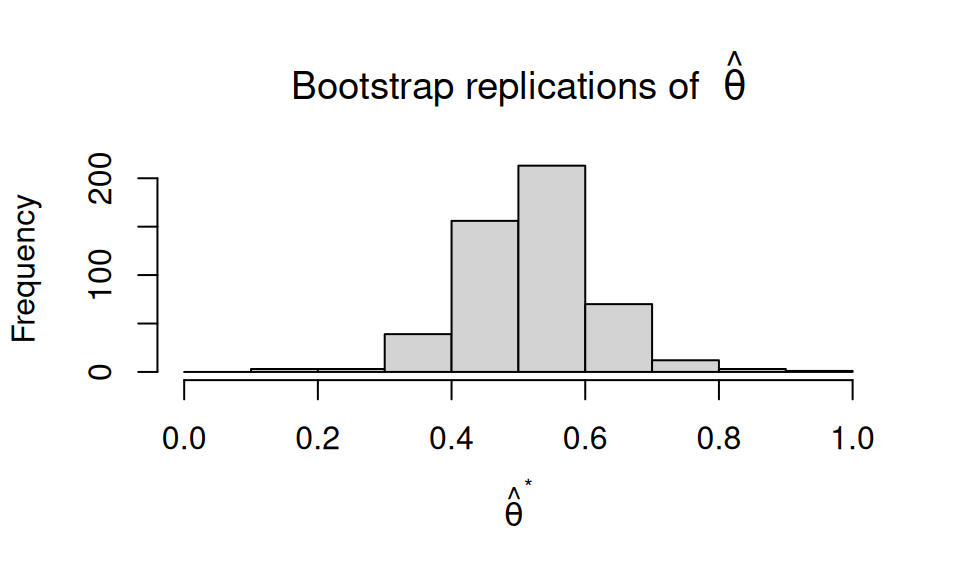
Figure 5.3: Bootstrap replications

5.4 Going Parallel

We are now ready to take what we’ve learned and parallelize the computation. In doing this we must be careful to follow the advice of Chapter 2 and use independent streams while sharing the load equally across processes. The set_up list constructed in sim_template that will be passed to the regression worker function ensures these conditions are satisfied.

Expanding on what we did with our example data set suggests that an appropriate worker function for the segmented regression model might look like

worker <- function(n, set_up, ...) {
  
  # unbundle the simulation parameters
  n_reps   <- set_up$n_reps
  stream_1 <- set_up$stream[[1]]
  stream_2 <- set_up$stream[[2]]
  seed_1   <- set_up$seed[[1]]
  seed_2   <- set_up$seed[[2]]
  
  # set the seed and stream
  dqset.seed(c(seed_1, seed_2), c(stream_1, stream_2))
  
  # unpack the model parameters
  param_list <- list(...)
  theta  <- param_list[[1]]
  sigma  <- param_list[[2]]
  beta_1 <- param_list[[3]]
  beta_2 <- param_list[[4]]
  B      <- param_list[[5]]
  
  # generate normal errors with replications in columns
  epsilon <- matrix(dqrnorm(n * n_reps, mean = 0, sd = sigma), 
                    nrow = n, ncol = n_reps)
  
  # independent variable
  t <- (1:n) / n
  
  # error sum-of-squares function
  SSE <- function(theta, y, t) {
    X_theta <- cbind(t * (t <= theta), t * (t > theta))
    reg_fit  <- lm.fit(X_theta, y)
    sum(reg_fit$residuals^2)
  }
  
  # carry out the simulation one replication at a time
  result <- apply(epsilon, MARGIN = 2, FUN = function(error) {
      # create the response data
      y <- beta_1 * t * (t <= theta) + beta_2 * t * (t > theta) +
           error
      
      # search for a starting value
      trial_values <- dqrunif(100)
      theta_start <- trial_values[which.min(sapply(trial_values,
                     SSE, t = t, y = y))]
      
      # estimate the breakpoint
      theta_hat <- optim(theta_start, SSE, y = y, t = t,
                   method = "Brent", lower = 0, upper = 1)$par
      
      # obtain residuals and fitted values
      X_hat <- cbind(t*(t <= theta_hat), t*(t > theta_hat))
      
      reg_fit <- lm.fit(X_hat, y)
      
      e   <- reg_fit$residuals
      fit <- reg_fit$fitted.values
      
      # collect the bootstrap estimates
      theta_hat_star <- numeric(B)
      
      for (b in seq_len(B)) {
        # construct bootstrap data
        y_star <- fit + dqsample(e, n, replace = TRUE)
        
        # search for a starting value
        trial_values <- dqrunif(100)
        theta_start <- trial_values[which.min(sapply(trial_values,
                       SSE, t = t, y = y_star))]
        
        # bootstrap estimate
        theta_hat_star[b] <- optim(theta_start, SSE, y = y_star,
                                   t = t, method = "Brent",
                                   lower = 0, upper = 1)$par
      }
      
      # estimator and bootstrap confidence interval
      c(theta_hat = theta_hat, 
        lower = quantile(theta_hat_star, 0.025, type = 1, 
                         names = FALSE),
        upper = quantile(theta_hat_star, 0.975, type = 1, 
                         names = FALSE))
    }
  )
  
  result
}

The first step in the above listing is to set the seed and increment of the generator using the information in set_up. Then, the model parameters are recovered from the ... argument. Next the array of random normal errors are created using dqrnorm. Each column of this matrix is then transformed into data from the change point model using the imported parameter values for the two slopes beta_1 and beta_2, the standard deviation sigma and the change-point theta. From there the sum-of-squares function is minimized using a 100 point blind random search for a starting value followed by an application of the Brent method in optim.

That brings us to the bootstrap step. The fit to the response vector and the vector of residuals are calculated and then used to create B bootstrap response vectors. For each one of these a corresponding bootstrap estimator theta_hat_star is calculated and the .025 and .975 percentiles of the resulting distribution are evaluated. This produces n_reps estimators of $\theta$ and their associated 95% bootstrap confidence intervals that are returned by the program.

5.5 An Exploratory Simulation Study

We used sim_template to investigate how the bootstrap confidence intervals performed in the context of our example data set with theta = .5, beta_1 = 1, beta_2 = 1.5, sigma = .25 with 4 cores. The basic experiment was replicated 500 times with 500 bootstrap samples:

sim_template(1234, 200, 500, 4, .5, .25, 1, 1.5, 500)

We also did this for $\theta$ = .8 and $\theta = .3$ with the same choices for the other parameters. Figure 5.4 shows histograms for $\hat\theta$ and Table 5.1 collects, for each change-point location, the median estimator value together with the coverage and the median length of the 95% bootstrap percentile interval.

The prospects for point estimation look encouraging at the three selected parameter values: the median estimates are 0.303, 0.501, and 0.802 and most of the action in the sampling distributions occurs at the true break point.

On the other hand the likelihood of normal approximations appears remote. The distributions are irregular, and their shapes depend strongly on the change-point location.

The bootstrap intervals are not uniformly calibrated: coverage is 0.888, 0.982, and 0.866. They overcover in the middle and undercover at the other two locations. The interval widths also change substantially, especially at $\theta=.3$.

What have we learned? Taken together, these experiments present a mixed but informative picture. The point estimator appears to locate the change point reasonably well at each of the three parameter values considered. Its sampling distribution, however, is distinctly non-normal and changes shape with the location of the change point. The residual-bootstrap intervals respond to that uncertainty, but their coverage is not reliably close to the nominal 95% level. These findings do not constitute a general assessment of either the estimator or the bootstrap procedure. They instead identify the next questions to investigate: sensitivity to the change-point location, sample size, noise level, and regression slopes, together with alternative interval procedures such as subsampling, an $m$-out-of-$n$ bootstrap, or methods designed specifically for nonregular change-point problems. In this sense, the simulation has done exactly what an exploratory study should do. It has separated an apparently promising point estimator from an interval-estimation problem that requires further work.

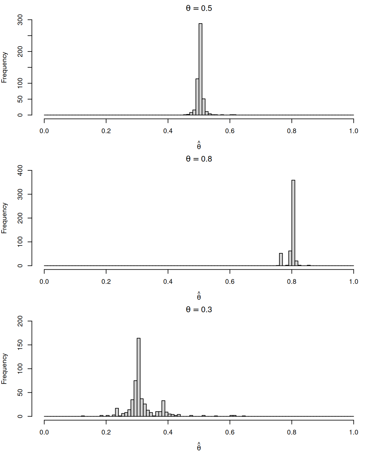
Figure 5.4: Histograms of change point estimators

Table 5.1: Bootstrap percentile interval performance across change-point locations. In every case $n = 200$ with 500 replications, $B = 500$ bootstrap resamples, and true slopes $\beta_1 = 1$, $\beta_2 = 1.5$ with $\sigma = .25$.
Change point	Median estimate	Coverage	Median length
0.3	0.303	0.888	0.246
0.5	0.501	0.982	0.043
0.8	0.802	0.866	0.050

Some timing runs were carried out for the regression change-point problem with theta = .5, beta_1 = 1, beta_2 = 1.5, sigma = .25 as before. We used samples of size 200 with 500 replications and 500 bootstrap samples. This produced the results in Table 5.2. These are median execution times across 10 consecutive runs. Here even the efficiency cores contributed to the speedup which was maximized when 8 processes were used on both machines. The relatively large one-process IQR on the iMac reflects a gradual increase in execution time across the ten runs rather than a single anomalous measurement.

Table 5.2: Table 5.3: Median elapsed execution times (seconds) for the parallel regression simulation. Interquartile ranges are shown in parentheses. Speedup is computed relative to the one-core execution on the same machine.
Cores	iMac M4 Median (IQR)	Speedup	ASUS i7 Median (IQR)	Speedup
1	738.66 (56.23)	1.00	685.72 (1.37)	1.00
2	403.58 (7.34)	1.83	340.36 (1.23)	2.01
3	299.46 (2.18)	2.47	238.79 (0.31)	2.87
4	240.27 (1.22)	3.07	182.16 (0.43)	3.76
5	202.36 (0.21)	3.65	155.94 (0.47)	4.40
6	179.42 (1.20)	4.12	137.99 (0.39)	4.97
7	170.42 (0.85)	4.33	124.43 (0.17)	5.51
8	167.06 (3.94)	4.42	115.98 (0.20)	5.91

5.6 Chapter Summary

In this chapter we put sim_template to work on a more substantive problem: esti- mating the change point in a segmented regression model. Standard large-sample theory does not suggest confidence interval formulas in this case and we instead tried a bootstrap approach.

The pattern that emerged in this chapter demonstrated how a real research question can be formulated to fit the parallel framework with minimal adjustment. The sim_worker function does the substantive work, data generation, estimation, and the residual bootstrap, while sim_template repeats it across processes. Simulation also gave us an avenue to fill the theoretical gaps. We empirically evaluated coverage rates and interval lengths across different parameter settings which showed us cases where the estimator worked well and where it did not.

Chapter 6 adapts the same machinery to a different problem: simulating an epidemic. There each replication is a stochastic process, not a parameter estimate. The processes do more than run independent copies; they represent interacting populations.

4 Parallel Simulation in Python

6 Case Study: Simulating an Epidemic in Python